
Preliminaries
In maximum entropy reinforcement learning, we have the objective
\[\begin{align} \mathcal J(\pi)=\sum_{t=1}^T\mathbb E_{s_{t}, a_{t}\sim \pi}\left[r(s_t,a_t)+\alpha\mathcal H(\pi(a_t|s_t))\right]\tag{1} \end{align}\]from which we can derive the following equivalence at the optimal piont
\[\begin{align} Q^\*(s_t,a_t)&=r(s_t,a_t)+\gamma\mathbb E_{p(s_{t+1}|s_t,a_t)}[V^\*(s_{t+1})]\tag{2}\\\ V(s_t)^\*&=\alpha\log\sum_{a}\exp\left({1\over\alpha}Q^\*(s_t,a_t)\right)\tag{3}\\\ \pi^\*(a_t|s_t)&=\exp\left({1\over\alpha}\Big(Q^\*(s_t,a_t)-V^\*(s_t)\Big)\right)\tag {4} \end{align}\]Plugging Eq.\((2)\) into Eq.\((4)\), we get
\[\begin{align} V^\*(s_t)-\gamma \mathbb E_{p(s_{t+1}|s_t,a_t)}[V^\*(s_{t+1})]=r(s_t,a_t)-\alpha\log\pi^\*(a_t|s_t)\tag {5} \end{align}\]We could generalize Eq.\((5)\) by adding consecutive time steps as follows
\[\begin{align} \mathbb E_{s_{t+1:t+d}|s_t,a_{t:t+d-1}}\left[\sum_{i=0}^{d-1}\gamma^{i}\big(V^\*(s_{t+i})-\gamma V^\*(s_{t+i+1})\big)\right]&=\mathbb E_{s_{t+1:t+d}|s_t,a_{t:t+d-1}}\left[\sum_{i=0}^{d-1}\gamma^{i}\big(r(s_{t+i},a_{t+i})-\alpha\log\pi^\*(a_{t+i}|s_{t+i})\big)\right]\\\ \mathbb E_{s_{t+1:t+d}|s_t,a_{t:t+d-1}}\left[V^\*(s_{t+i})-\gamma^{d}V^\*(s_{t+i+1})\right]&=\mathbb E_{s_{t+1:t+d}|s_t,a_{t:t+d-1}}\left[\sum_{i=0}^{d-1}\gamma^{i}\big(r(s_{t+i},a_{t+i})-\alpha\log\pi^\*(a_{t+i}|s_{t+i})\big)\right]\tag{6} \end{align}\]Path Consistency Learning
Based on Eq.\((6)\), Ofir Nachum et al. defines a notion of soft consistency error for a \(d\)-length sub-trajectory as
\[\begin{align} C(s_{t:t+d},\theta,\phi)=-V_\phi(s_t)+\gamma^dV_\phi(s_{t+d})+\sum_{i=0}^{d-1}\gamma^i\big(r(s_{t+i},a_{t+i})-\alpha\log\pi_\theta(a_{t+i}|s_{t+i})\big)\tag {7} \end{align}\]where the state value function and the policy are parameterized by \(\phi\) and \(\theta\), respectively. The goal of a learning algorithm is then to find \(V_\phi\) and \(\pi_\theta\) such that \(C(s_{t:t+d},\theta,\phi)\) is as close to \(0\) as possible for all sub-trajectories \(s_{t:t+d}\). Accordingly, Path Consistency Learning (PCL) attempts to minimize the squared soft consistency error over a set of sub-trajectories \(E\),
\[\begin{align} \mathcal L_{PCL}(\theta,\phi)=\sum_{s_{t:t+d}\in E}{1\over 2}C(s_{t:t+d},\theta,\phi)^2\tag {8} \end{align}\]This objective brings several benefits:
- We could replace both the policy and value function with \(Q\)-function since both could be represented by a \(Q\)-function as Eqs.\((3)\), \((4)\) suggested.
- The algorithm follows the actor-critic architecture, but this objective allows it to train in an off-policy fashion. This benefits from the fact that we do not maximize the expected rewards under the behavior policy here.
- It provides some theoretical guarantees of unbiased multi-step off-policy learning without importance sampling.
Algorithm
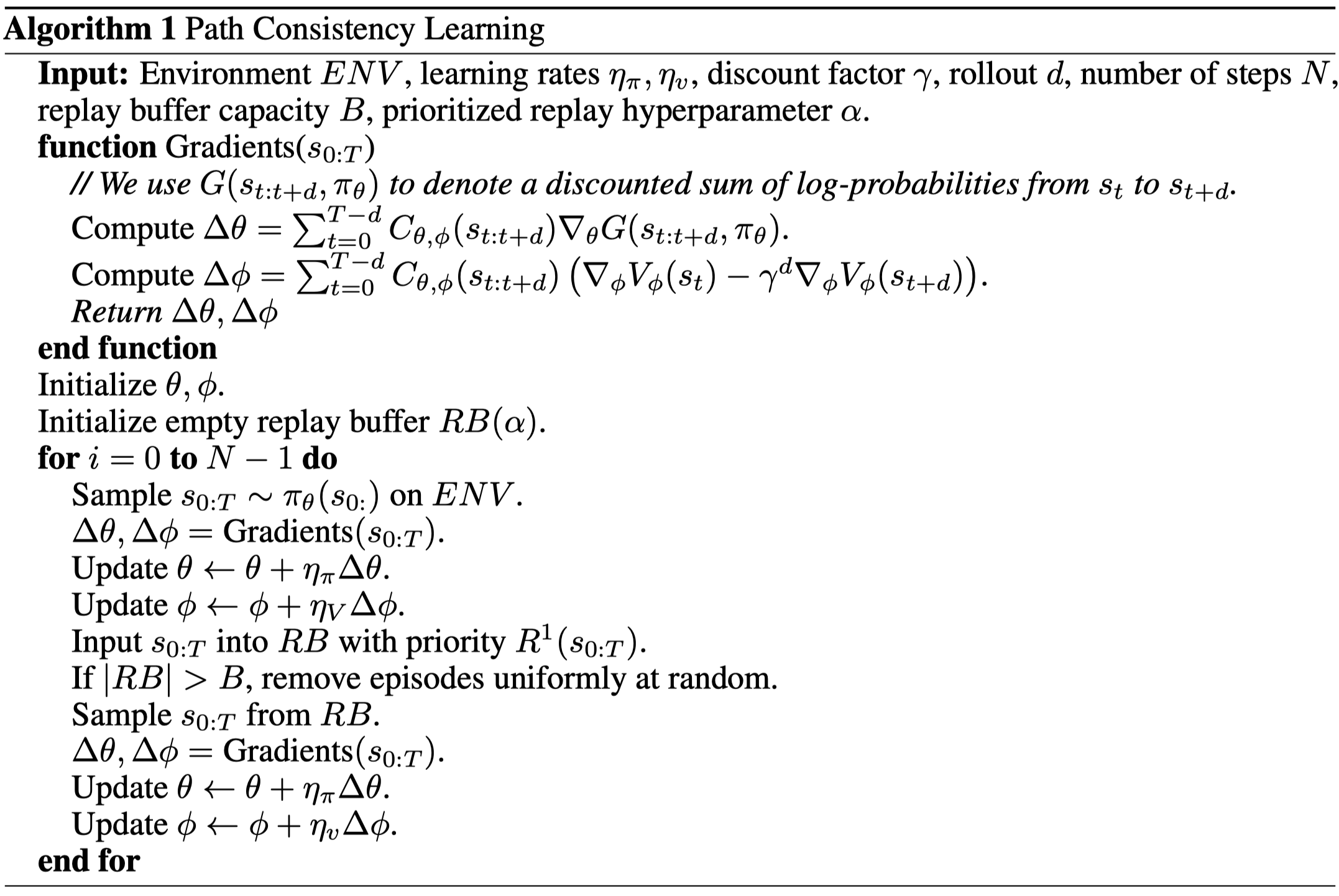
The algorithm learns from both on-policy and off-policy data. The off-policy sampling resembles prioritized experience replay, in which the authors propose to sample a full episode \(s_{0:T}\) from the replay of size \(B\) with probability \(0.1/B+0.9\exp(\alpha\sum_{t=0}^{T-1}r(s_t,a_t))/Z\), where \(Z\) is a normalization factor, and \(\alpha\) is a hyper-parameter. Moreover, there is no discounting on the sum of rewards.
Also, in practice, the authors find it beneficial to use a smaller learning rate for the value function than that for the policy.
Trust Path Consistency Learning
It’s been proven that small steps improve the stability and performance of policy-based methods. To gain these benefits, Ofir Nachum et al. in 2018 proposed adding constraints on PCL to avoid large step size, forming an algorithm named Trust Path Consistency Learning (Trust PCL).
In Trust PCL, we augment the maximum entropy objective defined in Eq.\((1)\) with a discounted relative entropy trust region
\[\begin{align} \mathcal J(\pi)=\sum_{t=1}^T\gamma^{t-1}\mathbb E_{s_{t}, a_{t}\sim \pi}\left[r(s_t,a_t)+\alpha\mathcal H(\pi(a_t|s_t))\right]\\\ s.t.\quad \sum_{t=1}^T\gamma^{t-1}D_{KL}(\pi(\cdot|s_t)|\pi_{old}(\cdot|s_t))\le\epsilon \end{align}\]Using the method of Lagrange multipliers, we cast this constrained optimization problem into maximization of the following objective
\[\begin{align} \mathcal J(\pi)&=\sum_{t=1}^T\gamma^{t-1}\mathbb E_{s_t,a_t\sim\pi}[r(s_t,a_t)-\alpha\log\pi(a_t|s_t)-\lambda\log\pi(a_t|s_t)+\lambda\log\pi_{old}(a_t|s_t)]\\\ &=\sum_{t=1}^T\gamma^{t-1}\mathbb E_{s_t,a_t\sim\pi}[\tilde r(s_t,a_t)+(\alpha+\lambda)\mathcal H(\pi(a_t|s_t))]\tag{9}\\\ where\quad&\tilde r(s_t,a_t)=r(s_t,a_t)+\lambda\log\pi_{old}(a_t|s_t) \end{align}\]where \(\pi_{old}\) in practice is denoted by a lagged policy \(\pi_{\tilde\theta}\), which is updated by \(\tilde\theta\leftarrow(1-\tau)\tilde\theta+\tau\theta\) at each training step. This objective(in fact, we have seen this objective back when we talk about iLQR with linear Gaussian models) is analogous to the objective defined in Eq.\((1)\), with different reward function and temperature. Therefore, following the same procedure as before, we derive the soft consistency error for a \(d\)-length sub-trajectory as
\[\begin{align} C(s_{t:t+d},\theta,\phi)=-V_\phi(s_t)+\gamma^dV_\phi(s_{t+d})+\sum_{i=0}^{d-1}\gamma^i\big(\tilde r(s_{t+i},a_{t+i})-(\alpha+\lambda)\log\pi_\theta(a_{t+i}|s_t+i)\big)\tag {10} \end{align}\]Adaptable \(\lambda\)
As it is in TRPO, \(\lambda\) in Eq.\((10)\) is in general harder to fine-tune than \(\epsilon\) in the constraint. The authors propose a sophisticated method, in which we set \(\epsilon\) beforehand and adapt \(\lambda\) accordingly during training. The inference procedure is trivial and based on many assumptions that are oftentimes not met in practice, but the resulting method works well in their experiments. Thus, we only present the method here with minimum explanation.
we perform a line search to find maximum \(\lambda\) that satisfies the following constraint
\[\begin{align} D_{KL}(\pi^\*\Vert\pi_{old})=-\log Z+\mathbb E_{s_{1:T}\sim\pi_{old}}\left[{R(s_{1:T})}\exp\big(R(s_{1:T})-\log Z\big)\right]<{\epsilon\over N}\sum_{k=1}^NT_k\\\ where\quad Z=\mathbb E_{s_{1:T}\sim\pi_{old}}\left[\exp\big(R(s_{1:T})\big)\right]\\\ R(s_{1:T})=\sum_{t=1}^Tr(s_t,a_t)/\lambda \end{align}\]where the LHS of inequality, which is under the expectation of \(\pi_{old}\), is approximated using the transitions from the last \(100\) episodes and \(T_k\) in the RHS is the length of episode \(k\).
References
Ofir Nachum et al. Bridging the Gap Between Value and Policy Based Reinforcement Learning
Ofir Nachum et al. Trust-PCL: An Off-Policy Trust Region Method for Continuous Control