
Introduction
We discuss OpenAI Five proposed by OpenAI et al., the first agent that defeats the Dota 2 world champion with some limitations.
I encourage anyone greatly interested in RL to read the paper—despite the length, it’s a well-written paper and relatively easy to follow. Here, I only excerpt some essential content that I’m personally interested in.
Table of Contents
- Training Details
- Observation Space
- Action Space
- Reward
- Architecture
- Exploration
- Surgery
- Experimental Results
Training Details
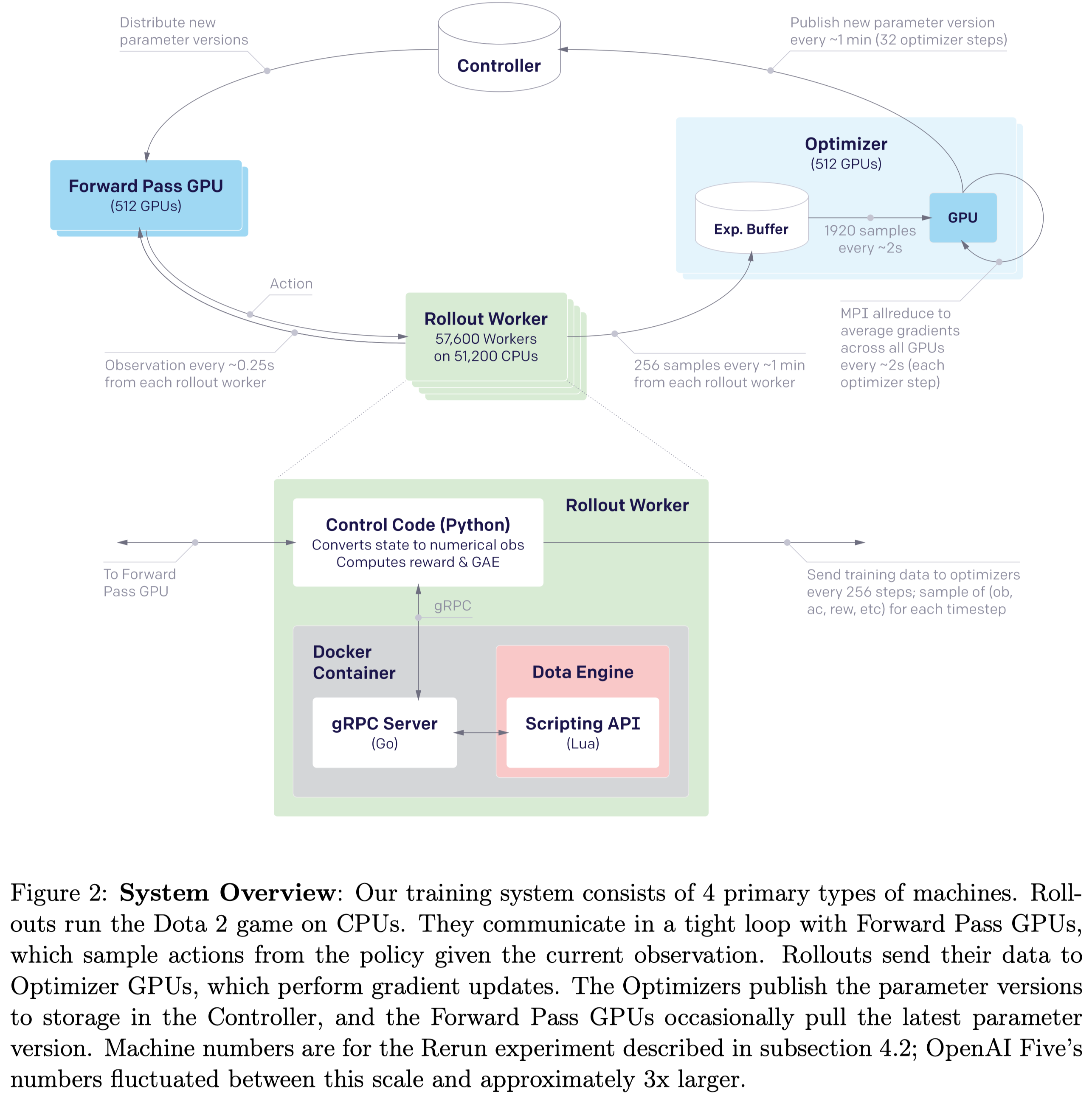
Figure 2 demonstrates the training system adopted by OpenAI Five. OpenAI Five uses 512 GPUs for inference and optimization, respectively. The experience buffer stores up to \(4096\) samples, each with \(16\) transitions. At the optimization step, each GPU fetches \(120\) samples from the buffer and computes gradient locally for all five hero policies. Gradients are averaged across the pool and clipped per parameter to be within \([-5\sqrt v,+5\sqrt v]\) before being synchronously applied to the parameters, where \(v\) is the running estimate of the second moment of the unclipped gradient. Every \(32\) gradient steps, the optimizers publish a new version of the parameters to a central Redis storage called the controller, which also stores all metadata about the state of the system, for stopping and restarting training runs.
Each worker plays the latest policy against itself for \(80\%\) of games and plays against older policies for \(20\%\) of games. A past version is selected proportional to its quality, which is initialized to the maximum existing qualities when an agent is added to the pool and slowly decreases when it’s defeated by the current agent. (Appendix H)
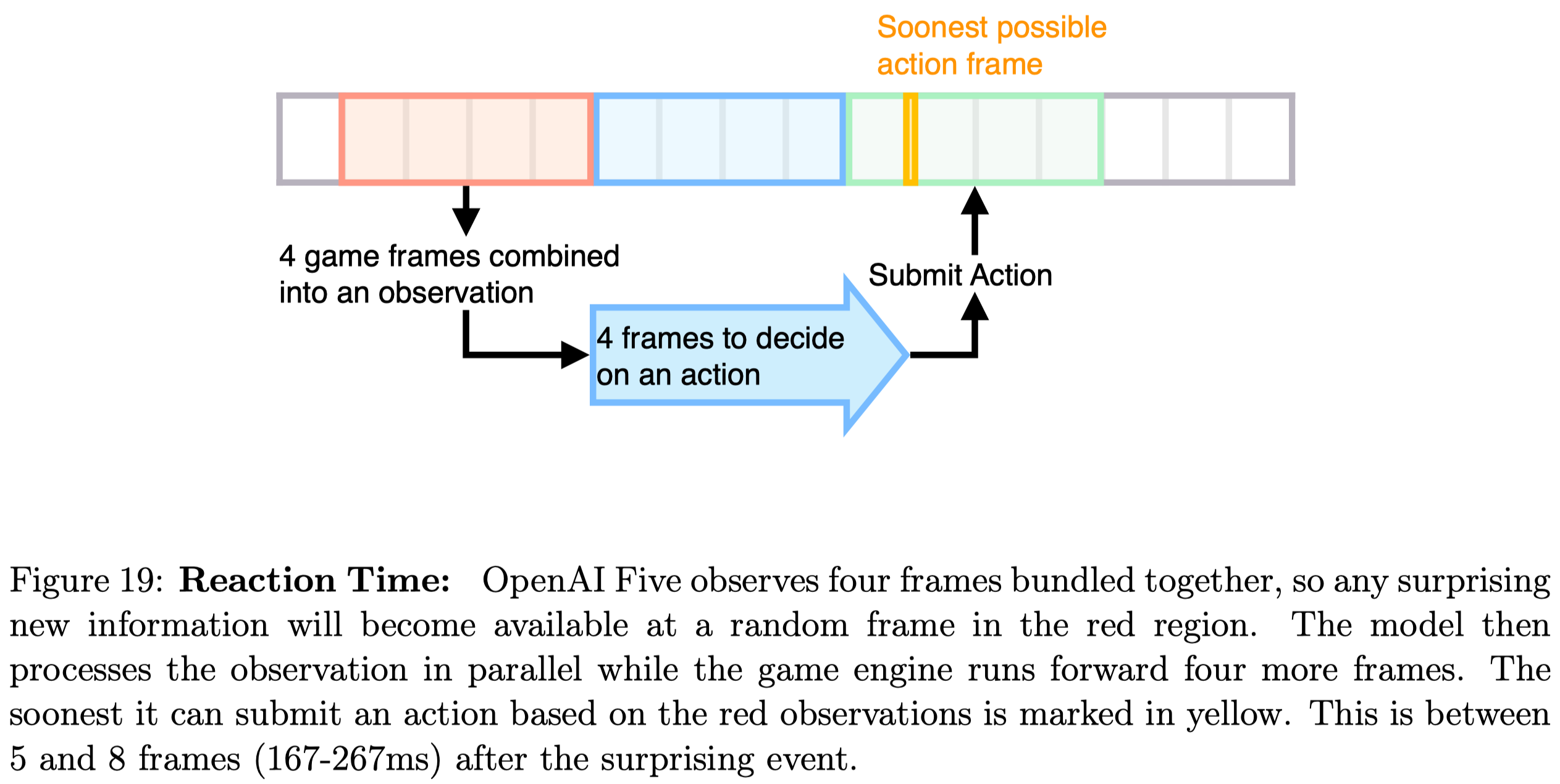
OpenAI Five reduces the computation requirements by allowing the game and the policy model to run concurrently by asynchronously issuing actions with an action offset. That is, when the model receives an observation at time \(T\), rather than making the game engine wait for the model to produce an action at time \(T\), they let the game engine carry on running until it produces an observation at \(T+1\). Then the game engine receives the action from the model produced at time \(T\) and proceeds accordingly. This prevents the two major computation from blocking one another (see Figure 19 below) but results in a reaction time randomly distributed between \(5\) and \(8\) frames (\(167\)ms to \(267\)ms)
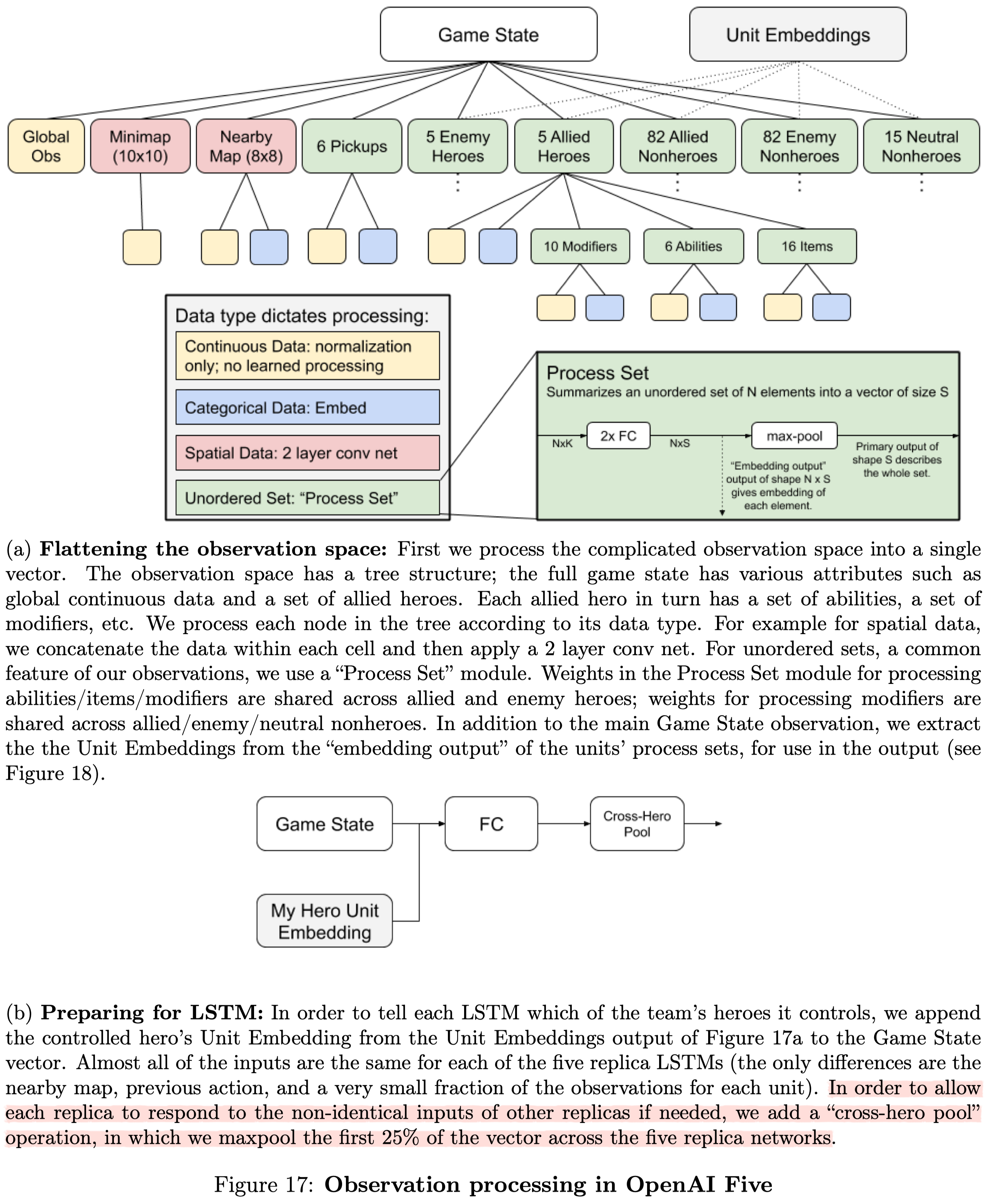
Observation Space(Appendix E)
OpenAI Five uses a set of data arrays to approximate the information available to a human player. This information is imperfect; there are small pieces of information which human can gain access to which is not encoded in the observation. On the flip side, the model gets to see all the information simultaneously every time step, whereas a human needs to actively click to see various parts of the map and status modifiers.
All float observations(including booleans) are z-scored using running mean and standard deviation before feeding into the neural network. This is done by subtracting the mean, dividing by the standard deviation, and clipping in range \((-5, 5)\) for each observation at each timestep.
Action Space(Appendix F)
The action that agents can choose at each timestep is represented by a primary action along with three parameter actions. The primary action includes noop, move, use one of the hero’s spell, etc. These actions are filtered by checking if it’s available before being fed into the network; as we will see in Architecture, the network is designed to accept a different number of available actions. Three additional parameter actions are delay(4 dim), unit selection(189 dim), and offset(81 dim) described in Figure 15 below. Interestingly, in Appendix L, they found that the agent did not learn to schedule delay, and simply taking the action at the start of the frameskip was better
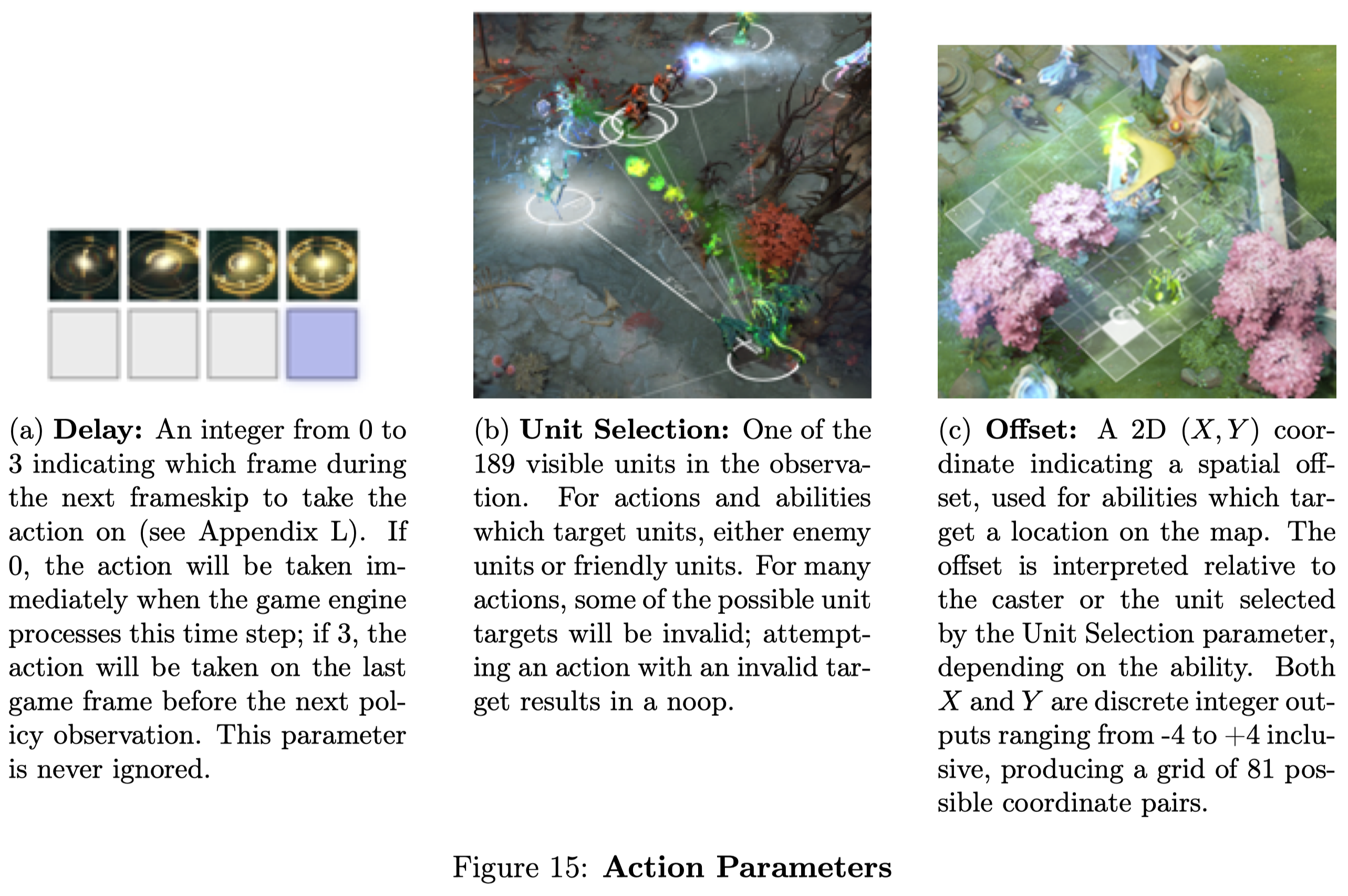
It is worth noting that Unit Selection is further divided into two heads depending on the primary action. One is Regular Unit Selection, which learns to target tactical spells and abilities, and the other is Teleport Selection, which repositions units across the map and is only activated when the primary action is teleport. Because teleport is much rarer, the learning signal for targeting this ability would be drowned out if we used a single head for both. For this reason, we separate them into two heads and use one or the other depending on the primary action. Similarly, the Offset parameter is split into “Regular Offset”, “Caster Offset” and “Ward Placement Offset”.
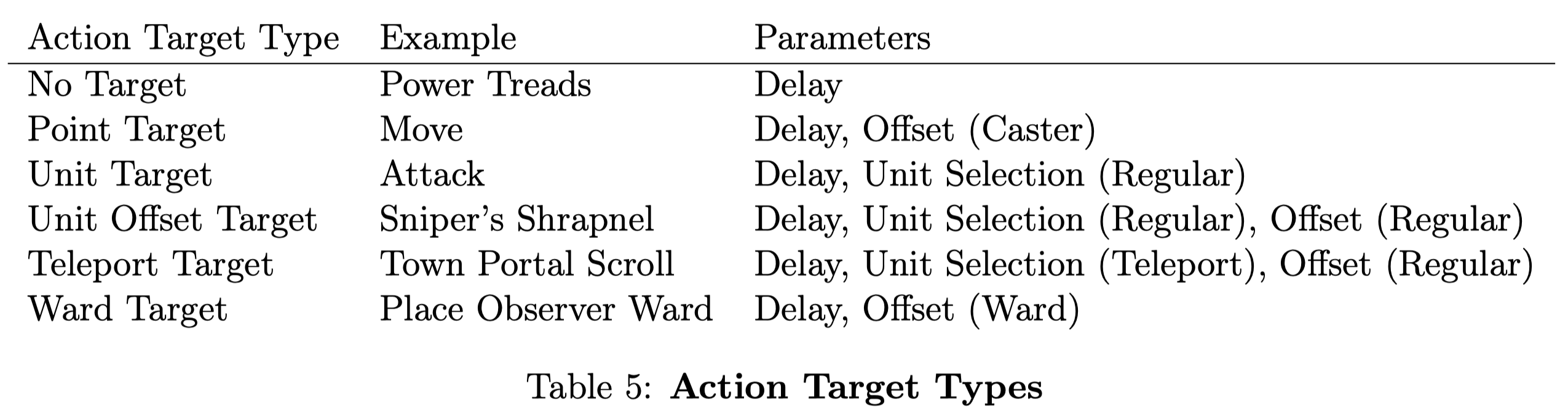
Table 5 categorizes primary actions into six action target types.
Reward(Appendix G)
To facilitate learning, a dense reward function is defined by human in addition to the win/loss signal. Instead of enumerating all rewards, we discuss three auxiliary techniques used in OpenAI Five:
Zero sum: To ensure all rewards are zero-sum, the average of the enemies’ rewards is subtracted from each hero’s reward
Game time weighting: Rewards are easily obtained in the late stage of the game as the hero’s power increases. For example, a character who struggles to kill a single weak creep early in the game can often kill many at once with a single stroke by the end of the game. If we do not account for this, the learning procedure focuses entirely on the later stages of the game and ignores the earlier stages because they have less total reward magnitude. To address this issue, we multiply all rewards other than win/loss reward by a factor that decays exponentially over the course of the game. Each reward \(\rho_i\) earned at time \(T\) is scaled:
\[\begin{align} \rho_i\leftarrow\rho_i\times 0.6^{T/10\text{mins}} \end{align}\]Team Spirit: As there are multiple agents on one team, the credit assignment problem becomes more intricate. This is further complicated as many rewards are given as team-based, in which case agents need to learn which of the five agent’s behavior causes these positive outcomes. OpenAI et al 2019 introduces team spirit \(\tau\) to measure how much agents on the team share in the spoils of their teammates. If each hero earns raw individual reward \(\rho_i\), the hero’s final reward \(r_i\) is computed as follows
\[\begin{align} r_i=(1-\tau)\rho_i+\tau\bar\rho \end{align}\]with scalar \(\bar\rho\) being equal to mean of \(\rho\). Although the final goal is to optimize for team spirit \(\tau=1\), they find that the lower team spirit reduces gradient variance in early training, ensuring that agent receives clearer rewards for advancing their mechanical and tactical ability to participate in fights individually.
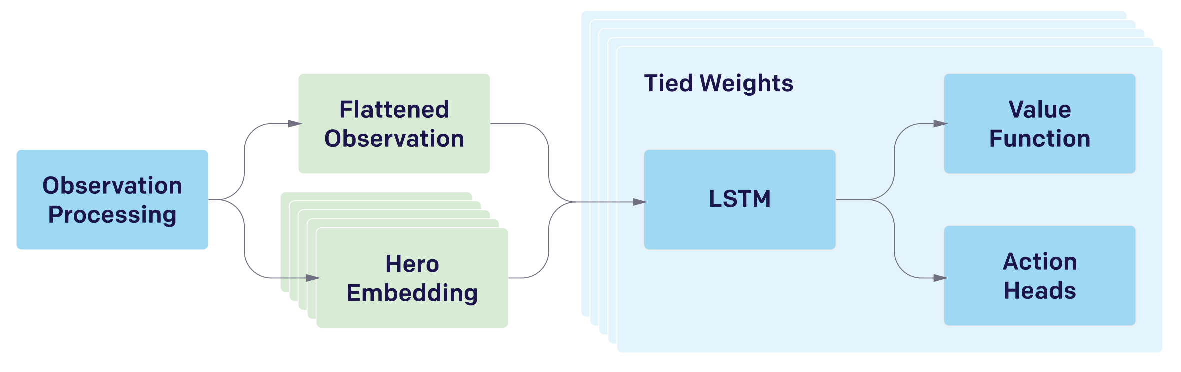
Architecture(Appendix H)
Separate replicas of the same policy function are used to control each of the five heroes on the team. This means that all heroes uses the same model, and the diversity is only introduced by the different observations and available actions. The following figures show the architecture from coarse to detailed
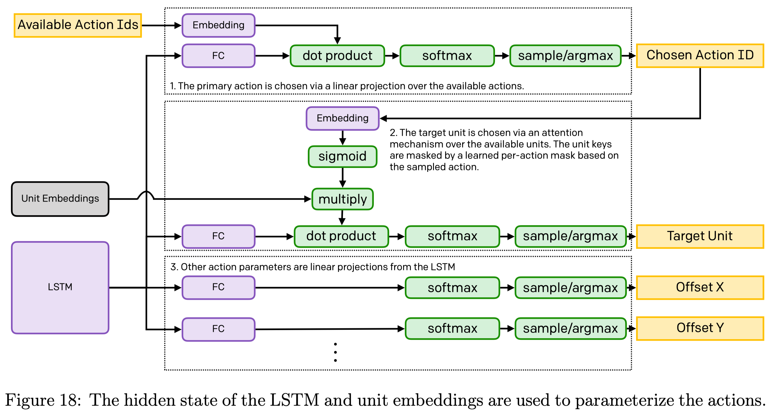
Target Unit Selection
The target unit selection is computed from two attention mechanisms:
- An action, such as attack, is first selected based on the cosine similarity between the embeddings of available actions and an output head from the LSTM. Assume \(H_a\in\mathbb R^{B\times W_a}\) is the output of the fully-connected layer in Figure18.1, and available action IDs are embedded in a matrix \(M\in\mathbb R^{N_a \times W_a}\), where \(B,W_a,N_a\) are the batch size, the embedding size, and the number of valid actions, respectively. We compute the softmax over the chosen action ID using
Theoretically, this design allows a varied number of available actions since the subsequent sample/argmax operation always yields a single action regardless of \(N_a\). In practice, however, if a batch contains a varied number of available actions, we still need mask to filter those unavailable actions(or maybe, we should separately process each element in the batch instead?).
- The chosen action ID is then embedded and multiplied by unit embeddings. The target unit is sampled/argmaxed from the dot product of this result and an output head of the LSTM. Let \(U\in\mathbb R^{N_u\times W_u}\) denote the unit embeddings, \(A \in\mathbb R^{1\times W_u}\) the action embedding, and \(H_u\in\mathbb R^{1\times W_u}\) the output of the fully-connected layer in Figure18.2, where \(N_u,W_u\) are the number of units(\(189\) according to the paper) and the embedding size, respectively. The softmax over the target units are computed as follows
where \(\circ\) is the Hadamard product. We can regard \(U\circ \sigma(A)\) as a gated linear unit, in which \(\sigma(A)\) modulates the information in the unit embedding \(U\) based on the action type. Therefore, \(H_u(U\circ \sigma(A))^\top\) computes the cosine similarity between the agent’s state \(H_u\) and the adjusted unit embeddings, \((U\circ \sigma(A))\), giving the scores that indicate how favorable each unit is based on the current agent state.
Exploration(Appendix O)
OpenAI et al. 2019 propose to encourage exploration in two different ways: by shaping the loss and by randomizing the training environment.
Loss Function
The loss function controls exploration in two ways: 1. The coefficient of the entropy bonus in PPO loss. 2. The team spirit discussed in the Reward section. A lower team spirit does better early in training, but it’s quickly overtaken by a higher one.
Environment Randomization
To further encourage exploration, OpenAI et al. 2019 identify three challenges in exploration:
- If a reward requires a long and very specific series of actions, and any deviation from that sequence will results in a negative advantage, then the longer this series, the less likely is the agent to explore this skill thoroughly and learn to use it when necessary.
- If an environment is highly repetitive, then the agent is more likely to find and stay in a local minimum.
- Agents must have encountered a wide variety of situations in training in order to be robust to various strategies humans employ. This parallels the success of domain randomization in transferring policies from simulation to real-world robotics
OpenAI et al. 2019 randomize to environments to address these challenges:
- Initial State: In rollout games, heroes start with random perturbations around the default starting level, gold, ability, etc.
- Lane Assignment: At a certain stage of their work, they noticed that agents developed a preference to stick together as a group of \(5\) on a single lane, and fighting any opponent coming their way. This represents a large local minimum, with higher short-term rewards but lower long-term ones as the resources from the other lanes are lost. After that, they introduced lane assignments, which randomly assigned each hero to a subset of lanes, and penalized them with a negative reward for leaving those lanes. However, the ablation study indicates that this may not be necessary at the end of the day.
- Roshan Health: Roshan(Similar to Baron in LOL) is a powerful creature, especially in the early games. Early in training agents were no match for it; later on, they would already have internalized the lesson never to approach this creature. To make this task easier to learn, Roshan’s health is randomized between zero and the full value, making it easier to kill.
- Hero Lineup: In each training game, teams are randomly sampled from the hero pool. An interesting observation is that the growing number of hero pool size only moderately slows down the training.
- Item Selection: Item selection is scripted in the evaluation, but in training, they are randomized around that.
Surgery(Appendix B)
OpenAI Five is a large project; it requires constant refinements to the training process, network architecture, etc. Furthermore, DOTA 2 is also updated regularly, changing the core game mechanics. It will be more efficient(in time and money) to refine the previous model instead of training a new model from scratch.
OpenAI et al. 2019 designed “surgery” tools for continuing to train a single set of parameters across changes to the environment, model architecture, observation space, and action space.
Changing the architecture and observation space: We discuss two situations: adding more units to a fully-connected layer and add more units to the LSTM layer. Notice that we can take changing the observation as a special case of the first situation. Suppose, we have two consecutive fully-connected layers:
\[\begin{align} y&=W_1x+B_1\\\ z&=W_2y+B_2\\\ \end{align}\]If we want to increase the dimension of \(y\) from \(d_y\) to \(\hat d_y\), it will cause the shapes of \(W_1, W_2, B_1\) to change. OpenAI et al. 2019 proposed to initialize the new variables as
\[\begin{align} \hat W_1=\begin{bmatrix}W_1\\\R()\end{bmatrix},\hat B_1=\begin{bmatrix}B_1\\\R()\end{bmatrix},\quad\hat W_2=\begin{bmatrix}W_2&0\end{bmatrix} \end{align}\]Where \(R()\) indicates a random initialization. The initialization of \(\hat W_1\) and \(\hat B_1\) ensure that the first \(d_y\) dimensions of activation \(\hat y\) will be the same as the old activation \(y\), and the remained will be randomized. The initialization of \(\hat W_2\), on the other hand, ensures that the next layer will ignore the new random activations, and the next layer’s activation will be the same as in the old model, i.e., \(\hat z=z\).
For LSTM, we cannot do the same because of its recurrent nature; if we randomize the new weights they will impact performance, but if we set them to zero then the new hidden dimensions will be symmetric and gradient updates will never differentiate them. OpenAI et al. 2019 finally decide to initialize new weights with random values significantly smaller than ordinary random initialization.
Changing the environment and action space: During experiments, OpenAI et al. 2019 spot that having the agent learn with new features might cause them to change a large portion of behaviors, which could significantly draw down the performance. Their solution is to make the agent play with both the old and new environment, and slowly increase the rate of the new environment.
Removing model parts: When some observation is removed, we simply set those to constants.
Smooth training restart: To ensure the gradient moments stored by the Adam optimizer are properly initialized when restarting with new parameters, the learning rate is set to \(0\) for the first several hours of training after surgery.
Moreover, because the rollout GPUs will be running the newest code, it is essential to ensure that past versions play at the same level after surgery—by going through the same “surgery” as the agent. Otherwise, past agents will forever play worse due to the change of the model, reducing the quality of the opponent pool.
Benefits: Surgery permits a tighter iteration loop for minor features and improvements.
Limits: Although “surgery” allows OpenAI Five to continually improve its performance in the face of changes, it’s still far from perfect. OpenAI et al. 2019 compared OpenAI Five, which went through a series of “surgery”, with Rerun, which was trained from scratch with the final version of the game and architecture. Rerun continued to improve beyond OpenAI Five’s skill and reached over \(98\%\) win rate against the final version of OpenAI Five.
Experimental Results
Data Quality
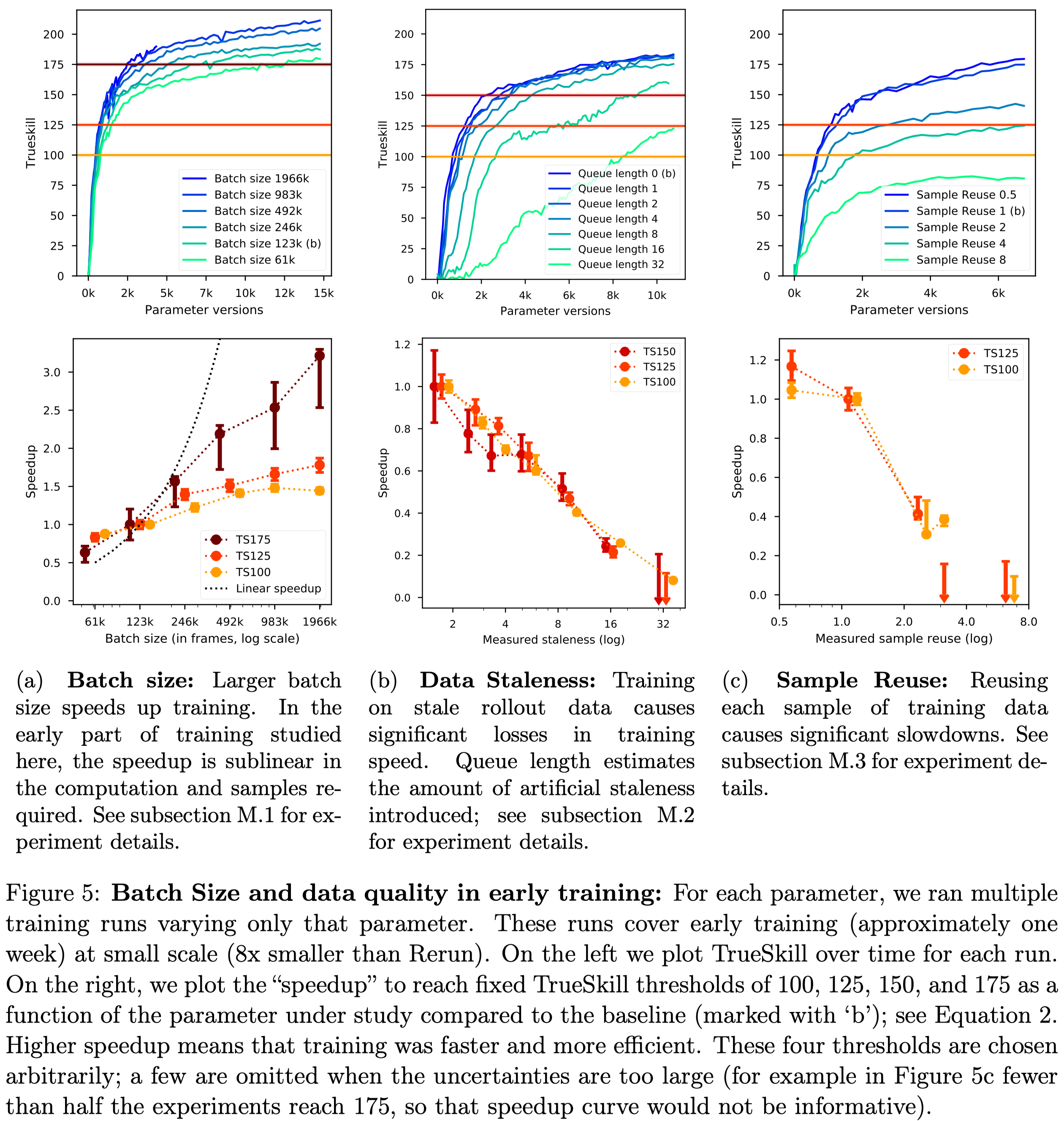
Figure 5a shows that a larger batch size can always speed up the learning process, but the performance gain slowly decreases when the batch size becomes large. On the other hand, data staleness and sample reuse can significantly slow down the training process. These results stress the important contribution of the on-policy data to the success of OpenAI Five.
Time Horizon
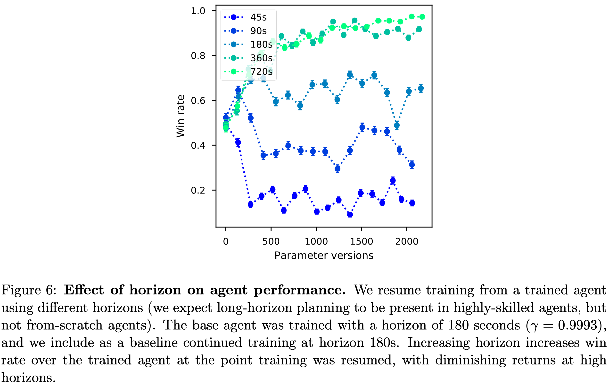
As Dota 2 has extremely long time dependencies, Open AI Five uses a time horizon up to \(360\) seconds, defined as
\[\begin{align} H={T\over 1-\gamma} \end{align}\]where \(H\) is the horizon, \(T\) is the real game time corresponding to each step(\(0.133\) seconds). When \(H=360\), \(\gamma\approx 0.99963\). Figure \(6\) shows the effect of the horizon on the agent performance.
References
OpenAI and Christopher Berner and Greg Brockman and Brooke Chan and Vicki Cheung and Przemysław Dębiak and Christy Dennison and David Farhi and Quirin Fischer and Shariq Hashme and Chris Hesse and Rafal Józefowicz and Scott Gray and Catherine Olsson and Jakub Pachocki and Michael Petrov and Henrique Pondé de Oliveira Pinto and Jonathan Raiman and Tim Salimans and Jeremy Schlatter and Jonas Schneider and Szymon Sidor and Ilya Sutskever and Jie Tang and Filip Wolski and Susan Zhang. 2019. “Dota 2 with Large Scale Deep Reinforcement Learning.” http://arxiv.org/abs/1912.06680.
OpenAI Blog: https://openai.com/blog/openai-five/