
Introduction
In the previous post, we have discussed a distributional deep Q network, namely c51. The c51 algorithm models the value distribution \(Z(s,a)\) using a discrete support \({z_1, \dots, z_N}\) uniformly spaced over a predetermined interval of return with respective atom probabilities represented by a parametric model \(\theta:S\times A\rightarrow \mathbb [0,1]^N\). This algorithm has the advantage of being highly expressive and computationally friendly, but it is restricted in practice since it requires the knowledge about the bounds of the return distribution. In this post, we will discuss two additional distributional deep Q networks that use a parametric model to estimate quantile values instead of probabilities.
Quantile Regression Deep Q Network
Why QR-DQN?
Quantile Regression Deep Q Network(QR-DQN) aims to solve the restriction of c51 by considering a fixed probability support instead of a fixed value support. Specifically, QR-DQN prescribes a discrete support taken on by the cumulative probability function (c.d.f.) and estimates quantiles of the target distribution via some parametric model. This inverse parametrization brings several benefits:
- We are not restricted to pre-specified bounds on the support (since the c.d.f. is in nature bounded in range \([0,1]\)), or a uniform resolution, potentially leading to significantly more accurate predictions when the range of returns vary greatly across state.
- It lets us do away with the unwieldy projection step present in c51 as there are no issues of disjoint supports. Together with \(1\), it obviates the need for domain knowledge about the bounds of the return distribution when applying the algorithm in practice.
- This reparametrization allows us to minimize the Wasserstein loss, without suffering from biased gradient, using quantile regression.
The Quantile Approximation
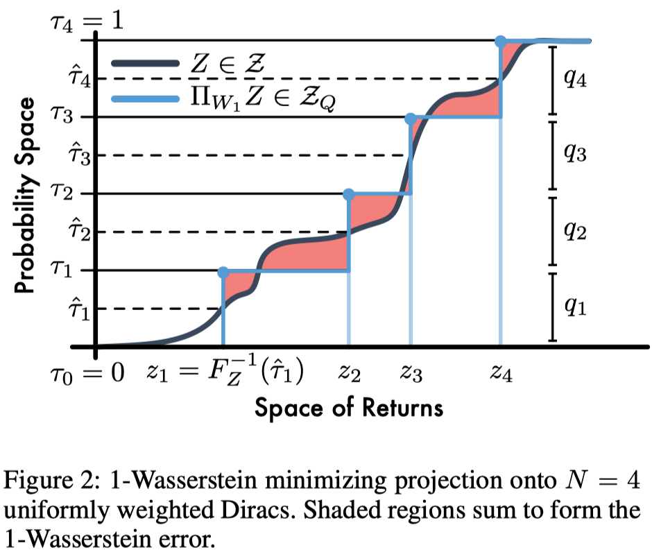
Let \(Z\) be an arbitrary value distribution with bounded first moment (e.g., \(\mathbb E_Z[X]=Q\) in our case), and \(Z_Q\) be the space of quantile distributions for fixed \(N\). We quantify the projection of \(Z\) onto \(Z_Q\) such that
\[\begin{align} \Pi_{W_1}Z:=\underset{Z_\theta\in Z_Q}{\arg\min}W_1(Z, Z_\theta) \end{align}\]where \(Z_\theta\) is a uniform value distribution over \(N\) Diracs with support \({\theta_1,\dots,\theta_N}\) (i.e., \(Z_\theta(s,a):={1\over N}\sum_{i=1}^N\delta_{\theta_i(s,a)}\)) and \(W_1\) is the 1-Wasserstein metric defined by
\[\begin{align} W_1(Z,Z_\theta)=\sum_{i=1}^N\int_{\tau_{i-1}}^{\tau_i}|F_Z^{-1}(\omega)-\theta_i|d\omega\tag{1} \end{align}\]where \(\tau_{i-1}\) and \(\tau_i\) are cumulative probabilities, and \(F_Z^{-1}\) is the quantile function (a.k.a., inverse cumulative distribution function) of \(Z\).
The following lemma shows how to compute the minimizer of Equation \((1)\)
Lemma: For any \(\tau,\tau’\in[0,1]\) with \(\tau<\tau’\) and cumulative distribution function \(F\) with inverse \(F^{-1}\), the set of \(\theta\in\mathbb R\) minimizing
\[\begin{align} \int_\tau^{\tau'}|F^{-1}(\omega)-\theta|d\omega \end{align}\]is given by
\[\begin{align} \left\{\theta\in\mathbb R\Bigg|F(\theta)=\hat\tau=\left(\tau+\tau'\over 2\right)\right\} \end{align}\]Proof: For any \(\tau,\tau’\in[0, 1]\) and \(\tau<\tau’\), we compute the sub-gradient of \(\int_\tau^{\tau’}\vert F^{-1}(\omega)-\theta\vert d\omega\) as follows
\[\begin{align} &{\partial\over\partial\theta}\int_\tau^{\tau'}|F^{-1}(\omega)-\theta|d\omega\\\ =&{\partial\over\partial\theta}\int_\tau^{\hat\tau}\theta-F^{-1}(\omega)d\omega+{\partial\over\partial\theta}\int_{\hat \tau}^{\tau'}F^{-1}(\omega)-\theta d\omega\\\ =&\hat\tau-\tau+\hat\tau-\tau'\\\ =&2\hat\tau-(\tau+\tau') \end{align}\]where \(\hat\tau=F(\theta)\in[\tau,\tau’]\) because \(F^{-1}\) is monotonically increasing and \(\int_\tau^{\tau’}\vert F^{-1}(\omega)-\theta\vert d\omega\) is convex. Setting this sub-gradient equal to \(0\) yields
\[\begin{align} \hat\tau=F(\theta)={\tau+\tau'\over 2} \end{align}\]which completes the proof.
Therefore, we can compute the minimizer of \(\theta\) by applying \(F^{-1}\) to both sides, which gives
\[\begin{align} \theta=F^{-1}\left({\tau+\tau'\over 2}\right) \end{align}\]This results in the minimizers of Equation \((1)\):
\[\begin{align} \theta_i&=F^{-1}_Z(\hat\tau_i)&\mathrm{for}\ i=1,\dots,N\tag{2}\\\ where\quad \hat\tau_i&={\tau_{i-1}+\tau_i\over 2} \end{align}\]So far we have showed that the quantile function \(\theta_i\) at \(\hat \tau_i=(\tau_{i-1}+\tau_i)/2\) minimizes the 1-Wasserstein metric defined in Eq.\((1)\). In the next section, we will see how to compute the quantile at a given point using a method named quantile regression.
Objective of QR-DQN
Quantile regression computes the quantile function by doing gradient descent on the quantile regression loss. The quantile regression loss, for quantile \(\hat\tau\in[0,1]\), is an asymmetric convex loss function that penalizes overestimation errors(\(\hat Z-\theta>0\) below) with weight \(\hat\tau\) and underestimation errors(\(\hat Z-\theta<0\) below) with weight \(1-\hat\tau\). Mathematically, we characterize the value of the quantile function \(F_Z^{-1}(\hat\tau)\) as the minimizer of the quantile regression loss:
\[\begin{align} \mathcal L_{QR}^{\hat\tau}(\theta)&:=\mathbb E_{\hat Z\sim Z}\left[\rho_{\hat\tau}(\hat Z-\theta)\right]\\\ where\quad \rho_{\hat\tau}(u)&:=u(\hat\tau-\mathbf 1_{u<0})\tag 3 \end{align}\]where \(Z\) is a value distribution and \(\hat Z\) is a value sampled from \(Z\). To avoid distraction, we do not further elaborate on the quantile regression loss; we refer interested readers to [3] and [4].
We generalize Equation.\((3)\) to obtain an objective that minimizes \({\theta_1,\dots,\theta_N}\) for \(W_1(Z,Z_\theta)\):
\[\begin{align} \mathcal L_{QR}^{\hat\tau}(\theta)&:=\sum_{i=1}^N\mathbb E_{\hat Z\sim Z}\left[\rho_{\hat\tau_i}(\hat Z-\theta_i)\right]\tag {4} \end{align}\]The quantile regression loss is not smooth at zero; as \(u\rightarrow 0^+\), the gradient of Equation \((3)\) stays constant. The authors hypothesized that this could limit performance when using non-linear function approximation. To this end, they also consider a modified quantile loss, called the quantile Huber loss. This quantile regression loss acts as an asymmetric squared loss in an interval \([-\kappa,\kappa]\) around zero and reverts to a standard quantile loss outside this interval:
\[\begin{align} \rho_{\hat\tau}^\kappa(u)&=|\hat\tau-\mathbf 1_{u<0}|\mathcal L_{\kappa}(u)\\\ where\quad \mathcal L_\kappa(u)&=\begin{cases}{1\over 2}u^2,&\mathrm{if\ }|u|\le\kappa\\\ \kappa(|u|-{1\over 2}\kappa),&\mathrm{otherwise}\end{cases} \end{align}\]In practice, we in general do not have access to the real target distribution \(Z\). As a result, the target distribution is approximated from the next state-action value distribution using the Bellman optimality operator. This yields the final loss function as follows
\[\begin{align} \mathcal L_{QR}^{\hat\tau}(\theta)&:=\sum_{i=1}^N\mathbb E_j[\rho_{\hat\tau_i}^\kappa(\mathcal T\theta_j-\theta_i)]= \sum_{i=1}^N{1\over N}\sum_{j=1}^N\rho_{\hat\tau_i}^\kappa(\mathcal T\theta_j-\theta_i)\tag {5}\\\ where\quad \mathcal T\theta(s, a)&:=r(s,a)+\gamma\theta(s',\arg\max_{a'}Q(s',a'))\\\ Q(s,a)&:=\mathbb E[\theta(s,a)]={1\over N}\sum_{i=1}^N\theta_i(s,a) \end{align}\]Note that there are two sums in Equation.\((5)\) (actually three, if we take into account the one in \(Q\) function): the first one sums over all probability supports, while the second approximates the expectation under the target distribution. Note that the latter works only because \(\hat\tau\) in Equation.\((2)\) uniformly spaced over the range of \([0,1]\).
Algorithm
Now we describe the algorithm, which basically follows Equation.\((5)\).
\[\begin{align} &\mathbf{Algorithm}\ \mathrm{QR\_DQN}(N, \kappa):\\\ 1.&\quad Q(s',a')=\mathbb E[\theta(s',a')]\\\ 2.&\quad a^\*=\arg\max_{a'}Q(s',a')\\\ 3.&\quad\mathcal T\theta_j(s,a)=r(s,a)+\gamma\theta_j^-(s',a^\*),\quad\forall j\\\ 4.&\quad\mathbf{output}\ \sum_{i=1}^N{1\over N}\sum_{j=1}^N\rho_{\hat\tau_i}^\kappa(\mathcal T\theta_j(s,a)-\theta_i(s,a)) \end{align}\]Note that we implicitly apply double DQN at step 1 by using \(\theta\) to compute the \(Q\)-value for the next time step, and, at step 3, we use the target network to approximate the target distribution.
Implicit Quantile Networks
Implicit Quantile Networks (IQN) extends QR-DQN from learning a discrete set of quantiles to learning the full quantile function, a continuous map from probabilities to returns. Taking an example from our previous discussion, to replicate the theoretical results of QR-DQN, we can have IQN take \(\hat\tau_i\) for \(i=1,\dots,N\) as the additional input and IQN will output the respective \(\theta_i\).
In practice, however, IQN does not take exact \(\hat\tau_i\) as QR-DQN does. Instead, IQN randomly samples a certain amount of probabilities from \(U([0, 1])\) at each time. Consequently, the IQN loss function becomes
\[\begin{align} \mathcal L_{IQN}&=\sum_{i=1}^N\mathbb E_{\tau'}\left[\rho_{\tau_i}^\kappa(\delta_t^{\tau_i,\tau_j'})\right]=\sum_{i=1}^N{1\over N'}\sum_{j=1}^{N'}\rho_{\tau_i}^\kappa(\delta_t^{\tau_i,\tau_j'})\tag {6}\\\ where\quad \delta_t^{\tau_i,\tau_j'}&=r_t+\gamma \theta_{\tau_j'}(s_{t+1},\pi_\beta(s_{t+1}))-\theta_{\tau_i}(s_t,a_t)\\\ \tau_i,\tau_j'&\sim U([0,1]) \end{align}\]where \(\theta_{\tau_i}\) outputs the quantile value at \(\tau_i\).
The freedom of the choice of \(\tau\) brings additional flexibility to the policy:
\[\begin{align} \pi_\beta(s) = \underset{a\in\mathcal A}{\arg\max}{1\over K}\sum_{k=1}^K\theta_{\tilde\tau_k}(s,a),\quad\tilde\tau_k\sim\beta(\tau),\ \tau\sim U([0,1])\tag {7} \end{align}\]where \(\beta:[0,1]\rightarrow[0,1]\) is known as a distortion risk measure, by choosing which we coud establish risk-sensitive behavior for the agent. Specifically, identity mapping corresponds to risk-neutral, concavity to risk-averse, and convexity to risk-seeking policies.
Note that the values of \(K\), \(N\), and \(N’\) could be different from each other, and the best values the authors found are \(K=32\), \(N=N’=8\).
Architecture

The architecture of IQN is comprised of three parts: \(\psi:\mathcal S\rightarrow \mathbb R^d\) encodes states (or more precisely, observations) into \(d\)-dimension vectors; \(\phi:[0,1]\rightarrow\mathbb R^d\) computes an embedding for the sample point \(\tau\); \(f: \mathbb R^d\rightarrow\mathbb R^{\vert \mathcal A\vert }\) maps the combination of \(\psi(s)\) and \(\phi(\tau)\) to the estimated action-values.
Some explanations:
-
\(\psi\) and \(f\) are the same functions as in DQN. Together, they consist of the quantile function.
-
\(\phi\) used by the authors, for embedding dimension \(n=64\), is defined as
which is just a fully-connected layer follow by ReLU with input vector \([\cos(\pi\tau),\dots,\cos(\pi n\tau)]\).
-
These functions are combined to form the approximation \(\theta_\tau(s,a)\approx f(\psi(s)\odot\phi(\tau))_a\), where \(\odot\) denotes the element-wise(Hadamard) product and is merely a design choice.
-
To gain some additional efficiency, we may run \(\phi(\tau_{1:N’})\) in parallel and tile \(\psi(s)\) as this implementation does.
Algorithm
\[\begin{align} &1.\quad\mathbf{Algorithm}\ \mathrm{IQN}(K,N,N',\kappa):\\\ &2.\quad\quad a^\*=\arg\max_{a'}{1\over K}\sum_{k=1}^K\theta_{\tilde\tau_k}(s',a'),\quad\tilde\tau_k\sim\beta(\cdot)\\\ &3.\quad\quad\tau_i,\tau_j'\sim U([0,1])\\\ &4.\quad\quad\delta_{ij}(s,a)=r(s,a)+\gamma\theta^-_{\tau_j'}(s',a^\*)-\theta_{\tau_i}(s,a),\quad\forall i,j\\\ &5.\quad\quad\mathbf{output}\ \sum_{i=1}^N{1\over N'}\sum_{j=1}^{N'}\rho_{\hat\tau_i}^\kappa(\delta_{ij}) \end{align}\]Some Interesting Experimental results
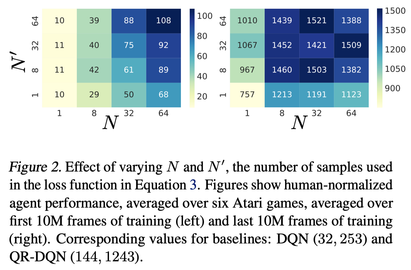
The above figure shows that both \(N\) and \(N’\) in Equation.\((6)\) have a dramatic effect on early performance, but neither has impact on the long-term performance past \(8\). Note that even for \(N=N’=1\), which is comparable to DQN in the number of loss components, the longer term performance is still quite strong (\(\approx 3\times\) DQN).
On the other hand, the authors did not find IQN to be sensible to \(K\) in Equation.\((7)\).
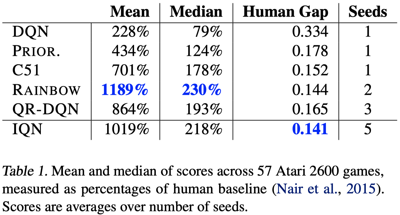
This figure shows that IQN performs better than all other single improvement on DQN. For games in which each algorithm continues to underperform humans(column 3), IQN outperforms all others including Rainbow, which is comprised of 6 improvements.
Comparison between QR-DQN and IQN
IQN provides several benefits over QR-DQN
- The approximation error for the distribution is no longer controlled by the number of quantiles output by the network, but by the size of the network itself, and the amount of training.
- IQN can be used with as few, or as many, quantile samples per update as desired, providing improved data efficiency with increasing number of samples per training update.
- The implicit representation of the return distribution allows us to expand the class of policies to risk-aware policies, taking advantage of the learned distribution.
Recap
In this post, we have discussed two algorithms based on quantile functions. When we talked about QR-DQN, we first derived the minimizers of 1-Wasserstein metric, the quantile functions \(\theta_i\) at \(\hat \tau_i=(\tau_{i-1}+\tau_i)/2\). Then we saw how quantile regression computes the quantile functions by doing gradient descent on the quantile regression loss, which gave us QR-DQN algorithm. Next, we discussed IQN, which dispenses with these predetermined discrete support. Instead, it directly learns the full quantile function and have probability \(\tau\) as a query input. This approach significantly improves the performance, and meanwhile, it allows the agent to pick up risk-sensitive policy by choosing \(\beta\) in Eq.\((6)\).
Discussion
Just as D4PG, one may combine QR-DQN or IQN with DDPG to yield an algorithm for continuous control problems.
References
- Will Dabney et al. Distributional Reinforcement Learning with Quantile Regression
- QR-DQN code by Arsenii Senya Ashukha
- Derivation of Quantile Regression
- Intuition of Quantile Regression
- Will Dabney et al. Implicit Quantile Networks for Distributional Reinforcement Learning
- IQN code from Google Dopamine