
Why Distributional DQN?
The core idea in distributional DQN is to model the value distribution \( Z(s,a) \), whose expectation is the action-value \( Q(s,a) \), i.e., \( Q(s,a)=\mathbb E[Z(s,a)] \). The benefits of modeling the distribution are
- An optimal \(Q^*\) may correspond to many value distributions, but only the one matching the full distribution of return under the optimal policy should be considered optimal. This suggests policies simply based on \(Q^*\) may be unstable, or chattering, and distributional value may reduce chattering.
- It helps to make better decisions if the environment is stochastic in nature compared to the general Bellman equation which takes advantage of expectation, ignoring the stochasticity in the environment.
- State aliasing may result in effective stochasticity due to partial observability, even in a deterministic environment. By explicitly modeling the resulting distribution, we provide a more stable learning target.
- The distributional approach naturally provides us with a rich set of auxiliary predictions, namely: the probability that the return will take on a particular value(\( z_i \)). However, the accuracy of these predictions is tightly coupled with the agent’s performance.
- Distributional DQN allows us to impose assumptions about the domain or the learning problem itself by choosing the support boundary \( [V_{\min}, V_{\max}] \). This enables us to change the optimization problem by treating all extremal returns as equivalent. Surprisingly, a similar value clipping in DQN significantly degrades performance in most games. On the other hand, this preknowledge about the domain may not always be available, which makes it fragile in many cases. Later we will discuss another two algorithms that bypass the this problem by considering probability supports.
- The KL divergence between categorical distributions is a reasonably easy loss to minimize.
- Sometimes even though the expected returns of 2 actions are identical, their variances might be different. Distributional methods gives us the space to choose between risk-seeking and risk-averse behavior by exploiting the value distribution, e.g. its variance.
The Distributional Bellman Equation
The value distribution can also be described by a recursive equation, the distributional Bellman equation:
\[\begin{align} Z(s,a)\overset{D}=R(s,a)+\gamma Z(S',A') \end{align}\]where the distributional equation \( U\overset{D}=V \) indicates that the random variable \( U \) is distributed according to the same law as \( V \). This equation states that the distribution of the return \( Z \) is characterized by the interaction of three random variables: the reward \( R \), the next state-action pair \( (S’, A’) \), and its next return \( Z(S’, A’) \).
There are several things worth being aware of:
- The Bellman’s expectation operator over value distributions is proved to be a contraction in a maximum form of the Wasserstein metric, but not in other metrics such as total variation, KL divergence. The corresponding proof will be outlined in Supplementary Material.
- The Bellman’s optimality operator over value distributions is not a contraction in any metric, i.e. no stable equilibrium is promised. These results provide evidence in favor of learning algorithms that model the effects of nonstationary policies.
- The distributional Bellman operator preserves multimodality in value distributions, which the authors believe leads to more stable learning. Approximating the full distribution also mitigates the effects of learning from a nonstationary policy. As a whole, this approach makes approximate reinforcement learning significantly better behaved.
Approximate Distribution Learning
Parametric Discrete Distribution
The value distribution is modeled by a discrete distribution parametrized by \( N\in \mathbb N \) and \( V_{\min}, V_{\max}\in \mathbb R \), and whose support is the set of atoms
\[\begin{align} \left\{z_i=V_{\min}+i\Delta z:0\le i<N\right\}\\\ \Delta z:={V_{\max}-V_{\min}\over N-1} \end{align}\]The corresponding atom probabilities are given by a parametric model \( \theta \): \( S\times A\rightarrow\mathbb R^N \).
\[\begin{align} Z_\theta(s,a)=z_i\\\ \mathrm{w.p.}\quad p_i(s,a):=\mathrm{softmax}(\theta_i(s,a))={\exp({\theta_i(s,a)})\over\sum_j\exp(\theta_j(s,a))} \end{align}\]The discrete distribution has the advantage of being highly expressive and computationally friendly (the regression loss, i.e., the MSE/huber loss on the \( Q \) value, is much more fragile and harder to optimize than an attribute classification loss).
Projected Bellman Update
Using a discrete distribution poses a problem: the Bellman update \( \mathcal {\hat T}Z_\theta \) and the original parametric value distribution \( Z_\theta \) almost always have disjoint support. To reexpress \( \mathcal {\hat T}Z_\theta \) in terms of the original support, we should project it back onto the support of \( Z_\theta \). For a given sample transition \( (s, a, r, s’) \), we compute each atom \( \mathcal{\hat T}z_j:=r+\gamma z_j \) (bounding it in the range of \( [V_{\min}, V_{\max}] \)), and then distribute its probability \( p_j(s’, \pi(s’)) \) to its immediate neighbour atoms in \( Z_\theta \) proportionally to their distances. If we regard each \( z_i \) as a bin and depict their probability as a histogram, this is the same general method how we project the values in between to its neighbouring bins.
The following equation computes the probability of \( \mathcal{\hat T}Z_{\theta} \) distributed to \( z_i \).
\[\begin{align} \left(\Phi \mathcal{\hat T}Z_\theta(s, a)\right)_i=\sum_{j=0}^{N-1}\left[1-{\left|\left[\mathcal{\hat T}z_j\right]_{V_{\min}}^{V_{\max}}-z_i\right|\over\Delta z} \right]_0^1p_j(s', \pi(s')) \tag {1} \end{align}\]where \( \left[\cdot\right]_a^b \) bounds its argument in the range \( \left[a, b\right] \).
At last, we view the parameter \( \theta \) in \( \mathcal {\hat T}Z_\theta \) as a fixed parameter \( \tilde \theta \), i.e., the parameters of the target network in DQN, and define the sample loss \( L_\theta(s,a) \) as the cross-entropy term of the KL divergence:
\[\begin{align} D_{KL}\left(\Phi\mathcal{\hat T}Z_{\tilde \theta}(s, a)\Vert Z_\theta(s,a)\right) \end{align}\]where \( \Phi\mathcal{\hat T}Z_{\tilde\theta}(s,a) \) is the projection of \( \mathcal {\hat T}Z_{\tilde\theta} \) onto the support of \( Z_\theta \). We do so since we expect \( Z_\theta (s,a) \) to be the optimal value distribution when it reaches the equilibrium.
The complete algorithm is shown as below.
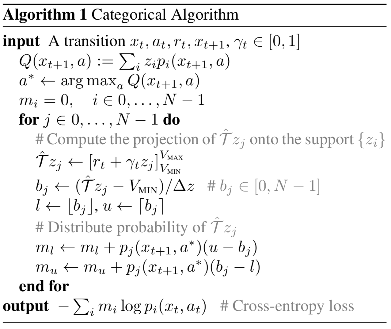
The computation process of the projection shown above leads to the same behavior as \( (1) \) indicates, only in a different manner:
- In each iteration, \( (1) \) computes the probability of \( \mathcal{\hat T}Z \) distributed to \( z_i \)
- In each iteration, the algorithm described above computes how the probability of \( \mathcal{\hat T}z_j \) is distributed to \( Z \)
Supplementary Materials
The Wasserstein Metric
The p-Wasserstein distance \( w_p \), which measures the similarity between two cumulative distribution funtions (c.d.f.), is the \( L_p \) metric on inverse cumulative distribution functions, also known as quantile functions. For random variables \( U \) and \( V \) with quantile functions \( F_U^{-1} \), \( F_V^{-1} \), respectively, it’s defined by
\[\begin{align} w_p(U,V):=\left(\int_0^1\left|F_U^{-1}(z)-F_V^{-1}(z)\right|^pdz\right)^{1/p} \end{align}\]where \(z\) denotes the cumulative probability. \( F^{-1}(z) \) is defined by \( F^{-1}(z)=\inf\left{x:F(x)\ge u\right} \), the smallest \( x \) with which the c.d.f. \( F(x) \) is greater than or equal to the probability \( z \).
Properties of The Wasserstein Metric
Consider a scalar \( a \) and a random variable \( A \) independent of \( U \) and \( V \). The metric \( w_p \) has the following property:
\[\begin{align} w_p(aU,aV)&\le|a|w_p(U,V)\\\ w_p(A+U, A+V)&\le w_p(U, V)\\\ w_p(AU, AV)&\le \Vert A\Vert_pw_p(U,V) \end{align}\]Proof of The Convergence of The Distributional Bellman Expectation in A Maximum Form of The Wasserstein Metric
In the prediction setting, define the maximal form of the Wasserstein metric:
\[\begin{align} \bar w_p(Z_1, Z_2)=\sup_{s, a}w_p(Z_1(s,a), Z_2(s,a)) \end{align}\]we’ll prove that the distributional Bellman expectation converges in \( \bar w_p \). Or in another word, \( \mathcal{\hat T}^{\pi}: \mathcal {Z\rightarrow Z} \) is a contraction in \( \bar w_p \).
\[\begin{align} \bar w_p(\mathcal{\hat T}^{\pi}Z_1, \mathcal{\hat T}^{\pi}Z_2)&=\sup_{s, a}w_p(\mathcal{\hat T}^{\pi}Z_1(s,a), \mathcal{\hat T}^{\pi}Z_2(s,a))\\\ &=\sup_{s, a}w_p(R(s,a)+\gamma P^{\pi}Z_1(s,a), R(s,a)+\gamma P^{\pi}Z_2(s,a))\\\ &\le\gamma \sup_{s,a}w_p(P^\pi Z_1(s,a), P^\pi Z_2(s,a))\\\ &\le\gamma \sup_{s',a'}w_p(Z_1(s', a'), Z_2(s', a'))\\\ &=\gamma \bar w_p(Z_1, Z_2) \end{align}\]where \( \mathcal{\hat T}^\pi \) is the Bellman operator: \( \mathcal{\hat T}^{\pi}Z(s,a)=R(s,a)+\gamma P^{\pi}Z(s,a) \). The first inequality follows from the properties of the Wasserstein metric, and the second follows the transition on \( Z \): \( P^\pi Z(s,a)\overset{D}{:=}Z(S’,A’) \)
References
Marc G. Bellemare et al. A Distributional Perspective on Reinforcement Learning