ICM, RND

Introduction

In reinforcement learning, the agent is trained to maximize the rewards designed to align with the task. The rewards are extrinsic to the agent and specific to the environment they are defined for. Most of the success in RL has been achieved when this reward function is dense and well-shaped. However, designing a well-shaped reward function is a notoriously challenging engineering problem. An alternative to “shaping” an extrinsic reward is to supplement it with dense intrinsic rewards, that is, rewards that are generated by the agent itself. Examples of intrinsic rewards include algorithms introduced in the previous post, such as exploration bonus and information gain exploration. In this post, we will first talk about another kind of an intrinsic rewards, namely curiosity, which uses prediction error as intrinsic reward signal. Then we will introduce an algorithm proposed by Burda et al.[3] named random network distillation that attempts to avoid some undesirable factors of prediction error in dynamic-based curiosity.

Dynamic-Based Curiosity

We formulate dynamic-based curiosity as the error in the agent’s ability to predict the consequence of its own actions. Directly predicting on the pixel level is tricky since the observation space is high and the agent will be overwhelmed by reconstructing every pixel in the image. Pathak et al[1]. propose predicting on a feature space learned by a self-supervised inverse dynamics model. The intuition is that the features learned should correspond to aspects of the environment that are under the agent’s immediate control.

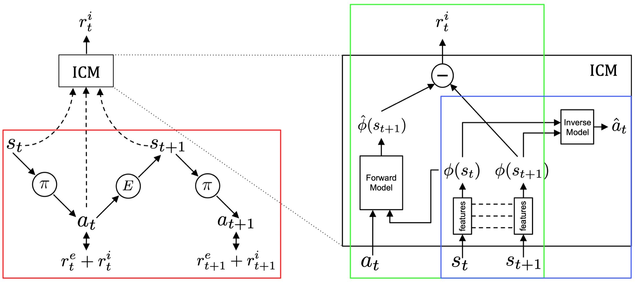
The above figure describes the architecture of the entire model. Now let us go through each part of them:

The part in the red box describes how the agent interacts with the environment. The policy here produces action based on the sum of extrinsic reward \(r^e\) provided by the environment and intrinsic reward \(r^i\) generated by the Intrinsic Curiosity Module(ICM).
The sub-module in the blue box illustrates the Inverse Dynamics Model(IDM), which describes how the feature space is learned. It takes as inputs states \(s_t\) and \(s_{t+1}\), and predicts the action \(a_t\). A potential downside could be that the features learned may not be sufficient. That is, they may not represent important aspects of the environment that the agent cannot immediately affect.
The sub-module in the green box describes how the intrinsic reward is generated. The current and the next states are first encoded by the encoding network, then we take as intrinsic reward the mean squared error between the predicted and real next state on the feature space.

Random Feature

The inverse dynamics model(IDM) mentioned in the previous section is effective, but it introduces another source of instability. That is, the feature extracted by IDM evolves as the model improved. One can avoid such instability by simply using a random embedding network that is fixed after initialization to encode the inputs. Although the resulting features in general fail to capture the important information, this method works decently well in practice thanks to its stability.

Death is Not The End

In episodic tasks, we generally have a ‘done’ signal to indicate the end of an episode. This could leak information about the task to the agent. To reinforce the bond between intrinsic rewards and pure exploration, Burda et al.[2] argue that the ‘done’ signal should be removed for pure exploration agent since the agent’s intrinsic return should be related to all the novel states that it could find in the future, regardless of whether they all occur in one episode or are spread over several. This suggests the discounted returns should not be truncated at the end of the episode and always bootstrapped using the intrinsic-reward value function. In practice, they do find that the agent avoids dying in the game since that brings it back to the beginning of the game, an area it has already seen many times and it can predict the dynamics well.

Random Network Distillation

The source of Prediction Error

Dynamic-based curiosity will be problematic when the dynamics is stochastic. A thought experiment named ‘noisy-TV’ problem describes this: an agent that is rewarded for errors in the prediction of its forward dynamics model easily gets attracted to local sources of entropy in the environment, such as a TV showing white noise. One could get rid of this problem by using methods that quantify the relative improvement of the prediction, rather than its absolute error. Unfortunately, such methods are hard to implement efficiently.

Burda et al.[3] identified three sources of prediction error:

Prediction error is high where the predictor fails to generalize from previously seen examples. Novel experience corresponds to this type of prediction error.
Prediction error is high because the prediction target is stochastic. Stochastic transitions are a source of such error for forward dynamics prediction
Prediction error is high because information necessary for the prediction is missing, or the model class of predictors is too limited to fit the complexity of the target function.

Factor 1 is useful since it quantifies the novelty of experience, whereas Factors \(2\) and \(3\) together cause the noisy-TV problem.

Structure

Random Network Distillation(RND) dispenses with the forward dynamics model to obviates Factors \(2\) and \(3\). Instead of predicting the next embedding feature from the current state and action, it predicts the output of a fixed randomly initialized neural network on the next state, given the next state itself. The following figure compares two methods

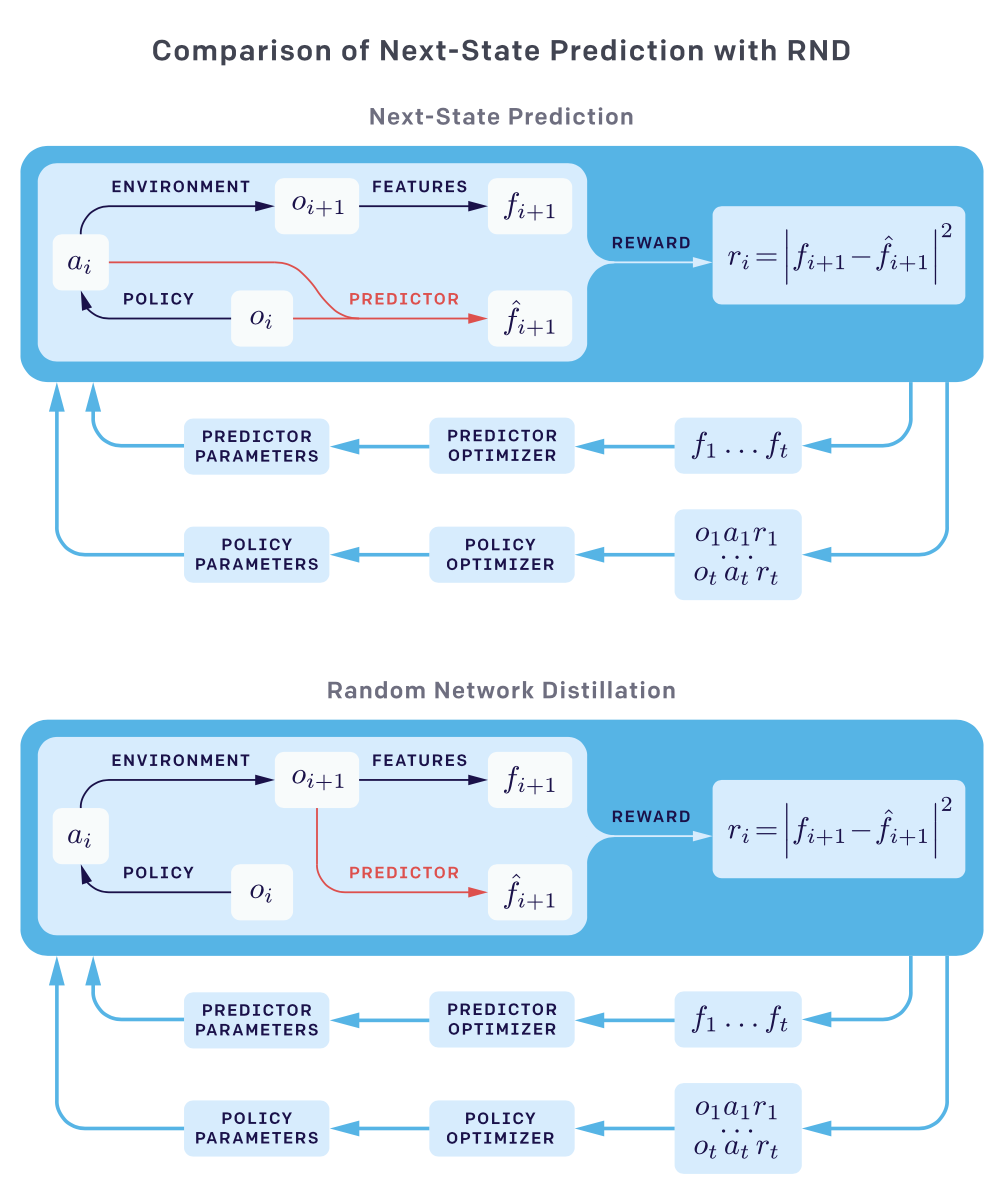
RND involves two networks: a fixed and randomly initialized target network \(f:\mathcal O\rightarrow \mathbb R^k\) that serves as the target of the prediction problem, and a predictor network \(\hat f:\mathcal O\rightarrow\mathbb R^k\) trained on the data collected by the agent to minimize the expected MSE \(\Vert \hat f(s;\theta)-f(s)\Vert^2\). This process distills a randomly initialized neural network into a trained one, and the prediction error is expected to be higher for novel states dissimilar to the ones the predictor has been trained on.

Before we move on, let’s take a step back to consider how this method get rid of Factors \(2\) and \(3\) we discussed before. RND forgoes the dynamics prediction so that it no longer concerns the transition dynamics and therefore avoids Factor 2. On the other hand, since the predictor network in practice has the same(or a larger) structure as the target network, indicating ideally these two networks could be perfectly matched, we do not need to worry about capacity issue described in Factor 3.

Combine Extrinsic and Intrinsic Returns

As discussed before, it is better to use non-episodic intrinsic return. In order to combine the episodic extrinsic and non-episodic intrinsic returns, the authors propose fitting two value heads \(V_E\) and \(V_I\) separately using their respective discounted returns, and combine them to give the value function \(V=V_E+V_I\). In their experiments, they use different discount factors, finding that \(\gamma_E=0.999\) and \(\gamma_I=0.99\) gives the best performance.

Algorithm

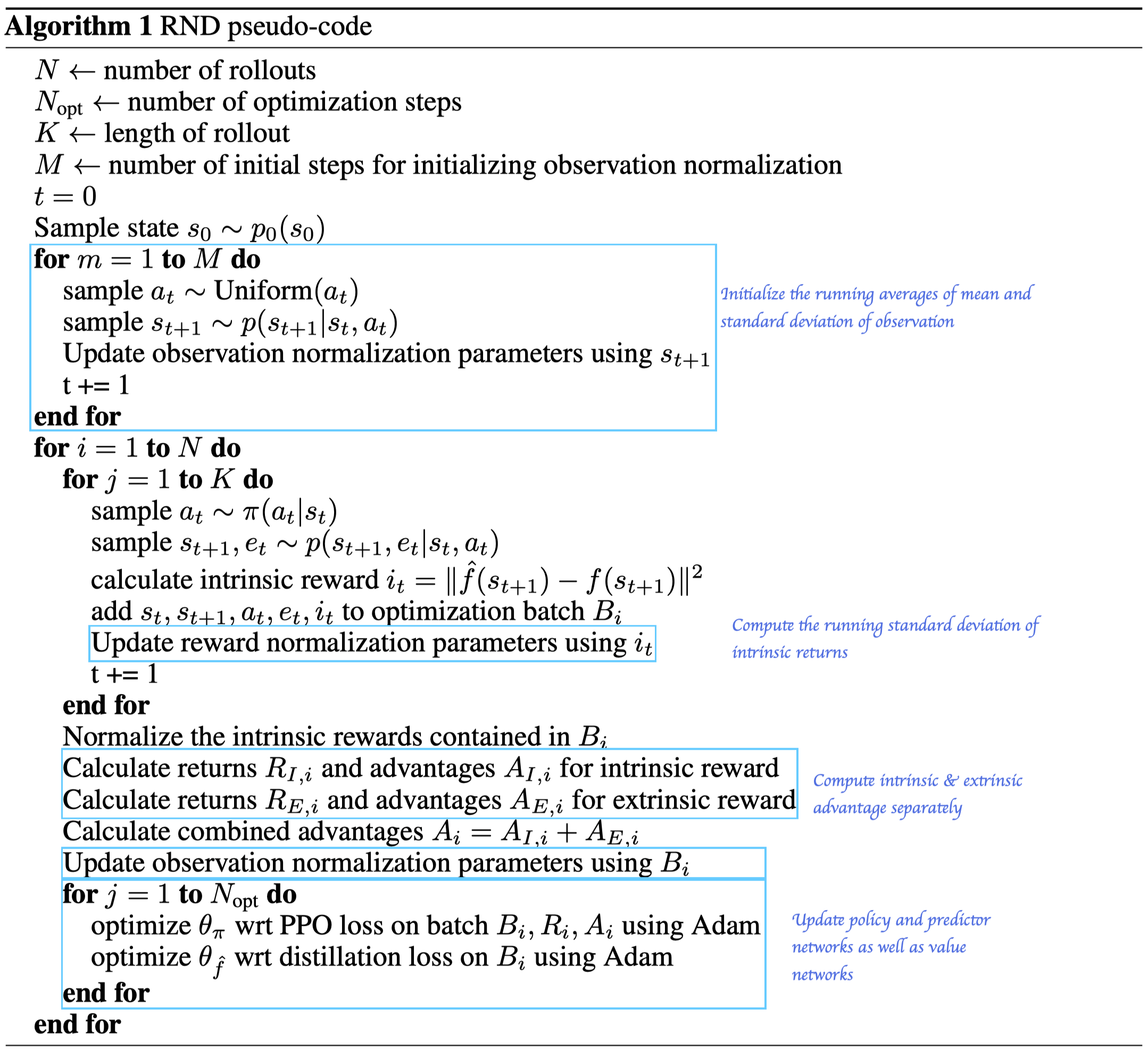
In practice, the authors suggest normalizing the intrinsic rewards by dividing it by a running estimate of the standard deviations(computed as this implementation) of the intrinsic return to keep the rewards on a consistent scale. Burda et al. also normalize observations to the target and predictor network by subtracting the running mean and then dividing by the running standard deviation and then the normalized observations are clipped to be between \(-5\) and \(5\). They do so since the target parameters are frozen and hence cannot adjust to the scale of different dataset. Lack of normalization can result in the variance of the embedding being extremely low and carry little information about the inputs.

Discussion

The RND exploration bonus is sufficient to deal with local exploration, i.e., exploring the consequences of short-term decisions, like whether to interact with a particular object or avoid it. However, a global exploration that involves coordinated decisions over long time horizons is beyond the reach of this method. To achieve these long-term exploration, it is often better to consider a systematic exploration method.

Reference

Deepak Pathak et al. Curiosity-driven Exploration by Self-supervised Prediction
Yuri Burda et al. Large-Scale Study of Curiosity-Driven Learning
Yuri Burda et al. Exploration by Random Network Distillation
RND code by OpenAI
https://openai.com/blog/reinforcement-learning-with-prediction-based-rewards/
https://www.endtoend.ai/slowpapers/exploration-by-random-network-distillation/``