
Introduction
Modern reinforcement learning algorithms have achieved astonishing results in many real-world games, such as Alpha Go and OpenAI Five. In this post, we discuss a more close-to-life application of reinforcement learning, known as web navigation problems, in which an agent learns to navigate the web following some instructions. Specifically, we discuss an algorithm, named QWeb proposed by Gur et al. ICLR 2019, that leverage DQN to solve web navigation problems.
Preliminaries
Simple Introduction to Web Navigation Problems
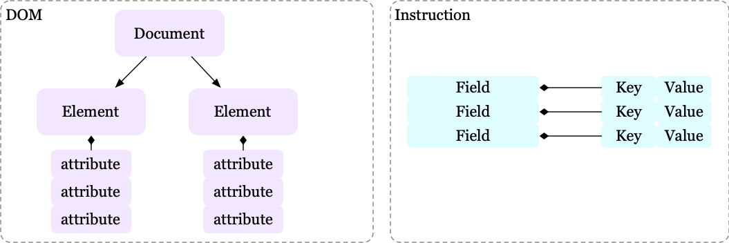
We first introduce two terminologies in web navigation problems:
- DOM is a tree representation of the web page, whose elements are represented as a list of named attributes.
- Instruction is a list of fields represented by key-value pairs.
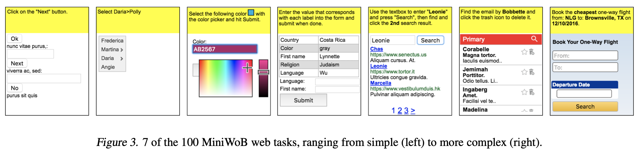
The agent’s objective is to navigate the web page(i.e., modify the DOM tree) such that it meets an instruction. The following figure demonstrates several MiniWoB web tasks:
Problem Setup

We first present the MDP \(\mathcal M=<\mathcal S, \rho, \mathcal A, \mathcal P,\mathcal R, \mathcal G, \gamma>\), where \(\rho\) denotes the initial state distribution, the transition function \(\mathcal P\) is deterministic, a goal \(\mathcal G\) is specified by the instruction, and \(\gamma\) is the discount factor. The rest notations are defined as follows:
- State space, \(\mathcal S\), consists an instruction and a DOM tree.
- Action space, \(\mathcal A\), contains two composite actions \(Click(e)\) and \(Type(e, y)\), where \(e\) is a leaf DOM element and \(y\) is a value of a field in an instruction. We further introduce three atomic actions to express these composite actions: \(a^D\) picks a DOM element \(e\), \(a^C\) specifies either a click or type action, and \(a^T\) generates a type sequence. Now we can represent \(Click(e)\) by \(a^D=e,a^C=\ ‘Click’\), and \(Type(e,y)\) by \(a^D=e, a^C=\ ‘Type’, a^T=y\).
- Reward, \(\mathcal R\), is a function of the final state of an episode and the final goal state. It’s \(+1\) if these states are the same, and \(-1\) if they are not. No intermediate reward is given.
QWeb
QWeb solves the above problem using deep \(Q\) network(DQN) to generate \(Q\) values for each state and for each atomic action. The training process is almost the same as traditional DQN with the help of reward augmentation and some curriculum learning approaches, which we will discuss later. But for now let’s first focus on the architecture of QWeb, which is essentially the most fruitful part of this algorithm.
Architecture
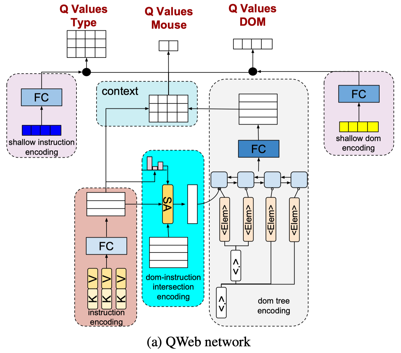
Encoding user instructions: As we’ve seen in the preliminaries, a user instruction consists of a list of fields, i.e.,key-value pairs \(<K, V>\). To produce a representation, we first encode words in keys, giving us \(f_K(i,j)\) for the \(j\)-th word in the key of \(i\)-th pair. Then we represent a key as the average of these embeddings, i.e. \(f_K(i)={1\over N}\sum_jf_{K}(i,j)\), where \(N\) is the number of words in the key. We also follow the same process to encode values, having embeddings \(f_V(i,j)\) and \(f_V(i)\). An instruction field is then produced by further encoding the concatenation of the key and value embedding through a fully-connected layer, i.e., \(f(i)=FC([f_K(i),f_V(i)])\), where \([\cdot]\) denotes vector concatenation. For now, we have encoded an instruction as \(f=Stack(f(i))\), a matrix whose rows are instruction fields.
Encoding DOM-Instruction Intersection: We first encode DOM element \(j\) by averaging the word embeddings over each sequence and each attribute, which gives us \(D(j)\). Then for each instruction filed \(f(i)\) and each element embedding \(D(j)\), we encode them through an encoder \(E(f(i),D(j))\). The conditional embedding of \(D(j)\) can then be expressed as the weighted average of these embedding, i.e. \(E_{cond}(j)=\sum_ip_iE(f(i), D(j))\), where probabilities \(p_i=softmax(u*f(i))\) with \(u\) being a trainable vector. One could take \(E_C\) as a self-attention module, where \(Q=u\), \(K=f\), and \(V=E(f,D)\).
Encoding DOM Trees: We concatenate the conditional DOM element embeddings \(E_{cond}(j)\) with DOM element embeddings \(D(j)\) to generate a single vector for each DOM element \(E_{conc}(j)=[E_{cond}(j), D(j)]\). Then we run a bidirectional LSTM(biLSTM) network on top of the list of DOM elements to encode the DOM tree. Each output vector of the biLSTM is then transformed through a fully-connected layer with tanh to generate DOM element representations, i.e., \(E_{tree}(j)=\tanh(FC(biLSTM(E_{conc}(j))))\).
Generating \(Q\) values: We compute the pairwise similarities between each field and each DOM element to generate a context matrix \(M=fE_{tree}^T\), where rows and columns of \(M\) show the posterior values for each field and each DOM element in the current state, respectively — notice that \(M[i][j]\) is the dot product of \(f(i)\) and \(E_{tree}(j)\)). We now use rows of \(M\) as the \(Q\) values for each instruction field, i.e, \(Q(s_t,a_t^T=i)=M[i]\). We compute the \(Q\) values for each DOM element by transforming \(M\) through a fully-connected layer and summing over the rows, i.e. \(Q(s_t,a_t^D)=sum(FC(M^T),1)\), where \(M^T\) is the transpose of \(M\). Finally, \(Q\) values for click and type actions on a DOM element are generated by transforming the rows of \(M\) into \(2\) dimensional vectors using another fully-connected layer, i.e., \(Q(s_t,a_t^C)=FC(M^T)\).
Incorporating Shallow Encodings: In scenarios where the reward is sparse and input vocabulary is large, such as in flight-booking environments with hundreds of airports, it is difficult to learn a good semantic similarity using only word embeddings. Gur et al. propose augmenting the deep \(Q\) network with shallow instruction and DOM tree encodings to alleviate this problem. For shallow encodings, we first define an embedding matrix of instruction field and elements as word-based similarities, e.g., Jaccard similarity, binary indicators such as subset or superset. Let’s take a concrete example to see what this embedding matrix looks like. Assuming the corpus of the instruction field consists of [“loc”, “date”, “name”], and that of DOM elements is comprised of [“name”, “loc”], the corresponding shallow encoding matrix looks like
\[\begin{align} \left[ \begin{array}{c|cc} &name&loc\\\ \hline loc&0&1\\\ date&0&0\\\ name&1&0 \end{array} \right] \end{align}\]A shallow input vector for DOM elements or instruction fields is generated by summing over columns or rows of the shallow encoding matrix, respectively. Take the above example; if we have an instruction field [“loc” “name”], then the resulting input vector is \([0, 1] +[1, 0]=[1,1]\). These shallow input vectors are then transformed using a fully-connected layer with tanh and scaled via a trainable variable to generates the corresponding shallow Q values. The final \(Q\) values are a combination of deep and shallow \(Q\) values
\[\begin{align} Q(s_t,a_t^D)=Q_{deep}(s_t,a_t^D)(1-\sigma(u))+Q_{shallow}(s,a_t^D)(\sigma(u))\\\ Q(s_t,a_t^T)=Q_{deep}(s_t,a_t^T)(1-\sigma(v))+Q_{shallow}(s,a_t^T)(\sigma(v)) \end{align}\]where \(u\) and \(v\) are scalar variables learned during training.
Reward Augmentation
So much for the architecture, now let’s shift our attention to the reward function. The environment reward function defined in the preliminaries is extremely sparse — the agent only gets a reward at the end of the episode, and worse still, the success states are a small fraction of the total state space, which makes the success reward even sparser. The authors therefore introduce a potential reward for remedy. Specifically, they define a potential function \(Potential(s,g)\) that counts the number of matching DOM elements between the current state \(s\) and the goal state \(g\). The potential reward function is then computed as the scaled difference between two potentials for the next state and the current state:
\[\begin{align} R_{potential}=\gamma(Potential(s_{t+1},g) - Potential(s_t,g)) \end{align}\]Curriculum Learning
The authors also propose two curriculum learning strategies to speed up the learning process:
- Warm-Start: To speed up the learning process, we warm-start an episode by choosing initial states somewhere near the goal state. These initial states can be obtained by randomly selecting a subset of DOM elements and having an oracle agent performs the correct action. The distance between the warm-started initial states and the goal state increases as the training progresses — which can easily be achieved by shrinking the selected subset.
- Goal Simulation: We also relabel states near the initial states as subgoals as done by HER, but here these states are generated by an oracle agent. As before, the distance between the subgoals and initial states increases as the training proceeds.
Notice that the above strategies are applied separately. Don’t mix them up.
Algorithm
\[\begin{align} &\mathbf{function}\ \mathrm{Curriculum\_DQN}:\\\ 1.&\quad\mathbf{for}\ each\ step\ \mathbf{do}:\\\ 2.&\quad\quad (I, D, G)\leftarrow\mathrm{sample\ instruction,\ initial,\ and\ goal\ states\ from\ environment}\\\ 3.&\quad\quad\mathrm{apply\ a\ curriculum\ strategy\ to\ modify}\ D\ \mathrm{or}\ (I,G)\\\ 4.&\quad\quad\mathrm{run\ DQN\_training}(QWeb,\ (D,\ I),\ G,\ env_w) \end{align}\] \[\begin{align} &\mathbf{function\ }\mathrm{DQN\_training}(Net,\ S,\ G,\ env):\\\ &//\ Train\ Net\ with\ set\ of\ initial\ states\ S,\\\ &//\ a\ goal\ state\ G,\ and\ environment\ env\\\ 1.&\quad\mathrm{run\ }Net(S)\ \mathrm{in}\ env\ \mathrm{to\ collect\ data,\ starting\ from\ }s\in S\\\ 2.&\quad\mathrm{compute\ potential\ reward}\ R_{potential}\ \mathrm{using\ }G\\\ 3.&\quad\mathrm{train\ }Net\ \mathrm{following\ DQN} \end{align}\]MetaQWeb
In the above method, we resort to an oracle agent to speed up the learning process in our sparse-reward problem, However, sometimes it is a luxury to have an oracle agent. For these cases, Gur et al. propose treating an arbitrary navigation policy as if it was an expert instruction-following policy for some hidden instruction. If we can recover the underlying instruction, we can autonomously generate new expert demonstrations and use them to do curriculum learning. Intuitively, generating an instruction from a policy is easier than following an instruction, as we don’t need the navigator to interact with a dynamic web page and take complicated actions. In this section, we first see how we create an arbitrary navigation policy, and then we present a way to infer the instruction for a given policy. We will put them all together in the end for completeness.
Note that I actually do not get this part of paper(Section 5) very well. I’ll leave my confusion whenever I think appropriate.
Rule-Based Randomized Policy(RBRP)
The rule-based randomized policy(RBRP, it’s named RRND by the authors for some obscure reason, we take this abbreviation for easy understanding) iteratively visits each DOM element in the current state and take action. It stops after all DOM elements are visited and returns the final state as goal state along with all intermediate state-action pairs. We take these state-action pairs as if they are generated by some optimal policy.
Instruction Generation Environment
To train an agent that infers instruction from a goal state, we define an instruction generation environment with the following attributes:
- We predefine a set of possible instruction keys for each environment
- The state space is comprised of a sampled goal and a single key in instruction sampled without replacement from the set of predefined keys.
- Instruction actions are composite actions comprised of 1) \(a^D\) which selects a DOM element, and 2) \(a^A\) which generate a value that corresponds to the current key.
- After each action, agent receives a positive reward (+1) if the generated value of the corresponding key is correct, otherwise a negative reward (-1). Initial and goal states are sampled using curriculum learning strategies as QWeb.
INET
INET takes as input an instruction key and a goal DOM tree, and output a full instruction for achieving the goal. This is done by sequentially fill in values for each key predefined by the instruction generation environment. Values are generated by a composite action: \(a^D\) finds a DOM element; \(a^A\) selects a DOM attribute from the element as the value. Next, we present the INET architecture.
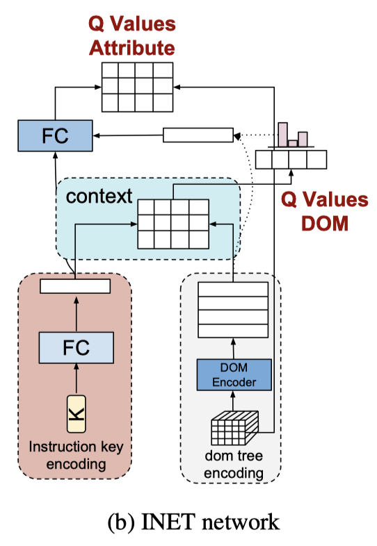
INET uses a similar structure as QWeb to encode instruction key and DOM tree, resulting in embedding \(f_K(i)\) and \(E_{tree}\) for the key and tree, respectively. We then compute the \(Q\) values for \(a^D\) as \(Q^I(s_t,a^D)=f_K(i)E_{tree}^T\) and \(Q\) values for \(a^A\) as \(Q^I(a,a^A, a^D=j)=FC([E_{tree}[j],f_K(i)])\), where \([.]\) denotes vector concatenation.
Algorithm
\[\begin{align} &\mathbf{function}\ \mathrm{MetaQWeb}\\\ 1.&\quad\mathbf{for\ }each\ step\ \mathbf{do}:\\\ 2.&\quad\quad(G, K, I)\leftarrow\mathrm{sample\ goal,\ key,\ instruction\ from\ instruction\ generation\ environment\ }env_I\\\ 3.&\quad\quad\mathrm{run\ DQN\_training}(INET,\ (G,K), I, env_I)\ \mathrm{to\ train\ } INET\\\ 4.&\quad\mathrm{fix\ }INET\mathrm{\ afterward}\\\ 5.&\quad\mathbf{for}\ each\ step\ \mathbf{do}:\\\ 6.&\quad\quad G,P\leftarrow \mathrm{run\ }RBRP\ \mathrm{get\ goal\ and\ state\ action\ pairs}\\\ 7.&\quad\quad\mathrm{using\ }P\mathrm{\ get\ a\ dense\ reward\ }R\\\ 8.&\quad\quad I\mathrm{\leftarrow run\ INET(G)\ to\ generate\ instruction}\\\ 8.&\quad\quad\mathrm{set\ up\ the\ environment\ }env_{DR}\ \mathrm{with\ new\ task\ }(I,G)\ \mathrm{and\ dense\ reward}\ R\\\ 9.&\quad\quad D\leftarrow\mathrm{sample\ initial\ state\ from\ }env_{DR}\\\ 10.&\quad\quad\mathrm{run\ DQN\_Training}(QWeb,\ (D,\ I),\ G,\ env_{DR}) \end{align}\]In MetaQWeb, RBRP randomly generates a goal and an ‘optimal’ policy achieving the goal from the current DOM state, then INET tries to find the underlying instruction that leads an agent to the goal. These are then fed to QWeb train our web navigation algorithm.
The dense reward may be some demonstration loss if we take the state-action pairs \(P\) as an optimal trajectory generated by some optimal policy. However, the authors seem to take the potential-based reward as described in the previous section.
Experimental Results
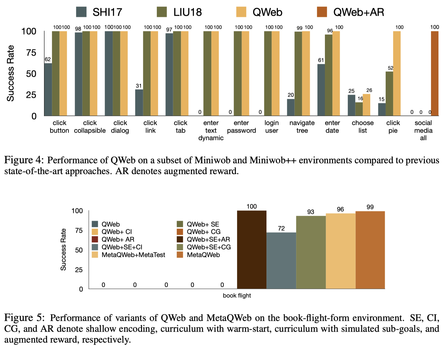
QWeb is able to exhibit outstanding performance during the experiments simply based on DQN.
Discussion
How does MetaQWeb speed up the training process of QWeb?
I’m not so sure if I take it correct. I personally think it boosts the training by provide more Instructions and goals. These goals may not be complete but can serve as subgoal to increase the training signals. Furthermore, we can apply warm-start as before by sampling the initial state from state-action pairs \(P\).
References
Izzeddin Gur, Ulrich Rueckert, Aleksandra Faust, Dilek Hakkani-Tur. Learning to Navigate the Web in ICLR 2019