
Introduction
As we’ve been coverd in the previous post, SAC exhibits state-of-the-art performance in many environments. In this post, we further explore some improvements on SAC.
Preliminaries
Back when we talked about Soft Value Iteration algorithm, we got the following update rules
\[\begin{align} Q(s_t,a_t)&=r(s_t,a_t)+\gamma\mathbb E_{p(s_{t+1}|s_t,a_t)}[V(s_{t+1})]\tag{1}\\\ V(s_t)&=\max_{\pi(a_t|s_t)} \mathbb E_{a_{t}\sim \pi(a_t|s_t)}[Q(s_t,a_t)+\alpha\mathcal H(\pi(a_t|s_t))]\tag{2}\\\ \pi(a_t|s_t)&=\exp\left({1\over\alpha}\Big(Q(s_t,a_t)-V(s_t)\Big)\right)\tag {3} \end{align}\]Then in this post, we derived objectives for SAC as follows
\[\begin{align} \mathcal L_Q(\theta_i)&=\mathbb E_{s_t,a_t, s_{t+1}\sim \mathcal D}\left[\big(r(s_t,a_t)+\gamma V_{\bar\psi}(s_{t+1})-Q_{\theta_i}(s_t,a_t)\big)^2\right]\quad \mathrm{for}\ i\in\{1,2\}\tag {4}\\\ \mathcal L_V(\psi)&=\mathbb E_{s_t\sim \mathcal D}\left[\big(\mathbb E_{a_t\sim \pi_\phi(a_t|s_t)}[Q_\theta(s_t,a_t)-\alpha\log \pi_\phi(a_t|s_t)]-V_\psi(s_t)\big)^2\right]\tag {5}\\\ \mathcal L_\pi(\phi)&=\mathbb E_{s_t\sim \mathcal D, \epsilon_t\sim \mathcal N}\left[\alpha\log \pi_\phi(f_\phi(\epsilon_t;s_t)|s_t)-Q_\theta(s_t,f_\phi(\epsilon_t;s_t))\right]\tag {6} \end{align}\]where we take \(Q_{\theta}=\min(Q_{\theta_1}, Q_{\theta_2})\) to mitigate the overestimation bias.
Removing Value Function
Later of Haarnoja&Zhou et al.’s work, they found the value function to be unnecessary, which came from the observation that Eq.\((6)\) does not rely on the value function. To remove the value function, we replace \(V\) in Eq.\((4)\) with Eq.\((2)\), which gives
\[\begin{align} \mathcal L_Q(\theta_i)&=\mathbb E_{s_t,a_t, s_{t+1}\sim \mathcal D}\left[\Big(r(s_t,a_t)+\gamma\mathbb E_{a_{t+1}\sim\pi_\phi(a_{t+1}|s_{t+1})}\big[Q_{\bar\theta}(s_{t+1},a_{t+1})-\alpha\log\pi_\phi(a_{t+1}|s_{t+1})\big]-Q_{\theta_i}(s_t,a_t)\Big)^2\right]\tag {7}\\\ &\qquad \mathrm{for}\ i\in\{1,2\}\\\ \end{align}\]where we \(Q_{\bar\theta}\) is the minimum of the target soft \(Q\)-functions that are obtained as an exponentially moving average of the soft \(Q\)-function weights. Noticeably, the official implementation does not choose \(a_{t+1}\) optimally. Instead, it samples \(a_{t+1}\) from the policy distribution, which is consistent with Eq.\((2)\).
Automating Entropy Adjustment for Maximum Entropy RL
SAC introduces an additional hypeparameter, namely temperature, to trade-off between entropy and reward maximization. Unfortunately, choosing the optimal temperature is non-trivial and the temperature needs to be tuned for each task. Hasrnoja&Zhou et al. later propose to automate the temperature learning by formulating a different MaxEnt-RL objective, where the entropy is treated as a constraint. Specifically, they propose finding a stochastic policy with maximal expectation return that satisfies a minimum expected entropy constraint as follows
\[\begin{align} \max_{\pi}\sum_{t=0}^T\mathbb E_{\pi}\left[r(s_t,a_t)\right]\\\ s.t.\mathbb E_{\pi}[-\log\pi(a|s)]\ge\mathcal H \end{align}\]where \(\mathbb E_{\pi}[-\log\pi(a\vert s)]\) computes the policy entropy and \(\mathcal H\) is a desired expected entropy—Haarnoja&Zhou et al. choose the negative of the dimension of the action space as \(\mathcal H\). To solve this constraint optimization problem, we reformulate it as the Lagrangian dual problem
\[\begin{align} \min_\alpha\sup_\pi\mathbb \sum_{t=0}^T\mathbb E_\pi\left[r(s_t,a_t)-\alpha(\log\pi(a_t|s_t)+\mathcal H)\right]\tag {8}\\\ s.t.\quad\alpha\ge0 \end{align}\]We can solve this problem by alternating between two steps:
- Maximize the objective \((8)\) w.r.t. \(\pi\)
- Minimizing the objective \((8)\) w.r.t. \(\alpha\)
We leave the detailed reasoning in the end. For now, let’s take a closer look at what these steps do: When we optimizing \((8)\) w.r.t. \(\pi\), it gives us exact the same MaxEnt RL objective as we use in SAC. Therefore, the first step is indeed performing gradient steps on SAC. The second step defines an additional objective for \(\alpha\):
\[\begin{align} &\min_\alpha\mathbb E_\pi[-\alpha(\log\pi(a_t|s_t)+\mathcal H)]\tag {9}\\\ =&\min_\alpha-\alpha(\mathcal H-\mathcal H_\pi),\quad where\ \mathcal H_\pi=-\mathbb E_\pi[\log\pi(a_t|s_t)] \end{align}\]This objective increases the temperature \(\alpha\) when the policy entropy is smaller than the target entropy and decreases the temperature \(\alpha\) when the policy entropy is larger than the target.
In practice, we found using \(\log\alpha\) in place of \(\alpha\) in Eq.\((9)\) yields better performance, i.e.
\[\begin{align} \min_\alpha\mathbb E_\pi[-\log\alpha(\log\pi(a_t|s_t)+\mathcal H)]\tag {10} \end{align}\]One possible explanation is that \(\log\alpha\) can be negative and is smoother when \(\alpha\) is small.
Algorithm
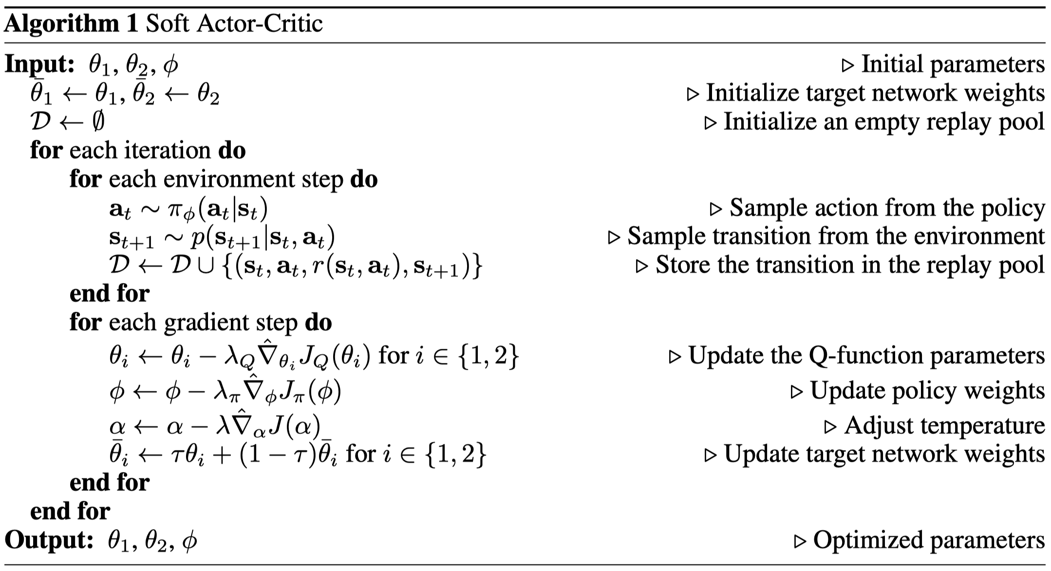
The algorithm does nothing more than what we described before.
Discussion
In the official implementation, the authors define the logarithm of the temperature as a single variable. This, however, universally penalize entropy for all state-action pairs, failing to distinguish different situations. We find it is helpful to make the temperature depend on state and action so that it exhibits different penalization to different state-action pairs.
Supplementary Materials
Dual Gradient Descent
For an optimization problem
\[\begin{align} \max f(x)\\\ s.t. g(x)\le 0 \end{align}\]the Lagrangian dual problem is defined as follows
\[\begin{align} \min_\lambda\sup_x\mathcal L(x,\lambda)\\\ s.t.\quad \lambda \ge 0\\\ where\quad \mathcal L(x, \lambda)=f(x)-\lambda g(x) \end{align}\]This problem can be solved by repeating the following steps
- We first find an optimal value of \( x \) that maximizes \( \mathcal L(x,\lambda) \), i.e., solving \( x^*\leftarrow\arg\max_x\mathcal L (x,\lambda) \)
- Then we apply gradient descent on \( \lambda \): \( \lambda \leftarrow \lambda - \alpha \nabla_\lambda \mathcal L(x^*,\lambda) \)
Now let us take a look at why this actually works. Note that \( -\lambda g(x) \) is non-negative when the constraint is satisfied since \( \lambda \ge0 \) and \( g(x)\le 0 \). Therefore, the Lagrangian \( \mathcal L(x,\lambda) \) is always an upper bound of \( f(x) \) as long as the constraint is satisfied, i.e.
\[\begin{align} \mathcal L(x,\lambda)\ge f(x) \end{align}\]Thus,
\[\begin{align} \sup_x(\mathcal L(x,\lambda))\ge \sup_x(f(x)) \end{align}\]As we continuously tune \( \lambda \) to minimize \( \sup_x(\mathcal L(x,\lambda)) \), \( \sup_x(\mathcal L(x,\lambda)) \) gradually approaches \( \sup_x(f(x)) \).
References
Haarnoja, Tuomas, Aurick Zhou, Kristian Hartikainen, George Tucker, Sehoon Ha, Jie Tan, Vikash Kumar, et al. 2018. “Soft Actor-Critic Algorithms and Applications.” http://arxiv.org/abs/1812.05905.