
Introduction
We show that the recent formulation introduced by Al-Shedivat et al. (2018) and Stadie et al. (2018) leads to poor credit assignment, while the MAML formulation (Finn et al., 2017) potentially yields superior meta-policy updates. Second, based on insights from our formal analysis, we highlight both the importance and difficulty of proper meta-policy gradient estimates. In light of this, we propose the low variance curvature (LVC) surrogate objective which yields gradient estimates with a favorable bias-variance trade-off. Finally, building upon the LVC estimator we develop Proximal MetaPolicy Search (ProMP), an efficient and stable meta-learning algorithm for RL. (excerpted from the Rothfuss, Lee&Clavera et al.[1])
Sampling Distribution Credit Assignment
Finn et al. proposed the objective of MAML-RL as follows
\[\begin{align} J^I(\theta)=&\mathbb E_{\mathcal T\sim\rho(\mathcal T)}\left[\mathbb E_{\tau'\sim P_{\mathcal T}(\tau'|\theta')}\left[R(\tau')\right]\right]\tag{1}\\\ where\quad\theta':=&U(\theta,\mathcal T)=\theta+\alpha\nabla_\theta\mathbb E_{\tau\sim P_{\mathcal T}(\tau|\theta)}[R(\tau)] \end{align}\]Al-Shedivat et al. and Stadie et al. proposed the following objective
\[\begin{align} J^{II}(\theta)=&\mathbb E_{\mathcal T\sim\rho(\mathcal T)}\left[\mathbb E_{\tau\sim P(\tau|\theta)\\\\tau'\sim P_{\mathcal T}(\tau'|\theta')}\left[R(\tau')\right]\right]\tag{2}\\\ where\quad\theta':=&U(\theta,\tau)=\theta+\alpha\nabla_\theta R(\tau) \end{align}\]The difference is that \(J^{II}(\theta)\) moves the expectation over \(\tau\) out of function \(U\) in \(J^I(\theta)\). This impact becomes clearer when we compute their gradients. Going through the math, we can compute the gradient of \(J^{I}(\theta)\) as follows
\[\begin{align} \nabla_{\theta}J^I(\theta)=\mathbb E_{\mathcal T\sim\rho(\mathcal T)}\Bigg[ \mathbb E_{\tau\sim P(\tau|\theta)\\\\tau'\sim P_{\mathcal T}(\tau'|\theta')} \bigg[\underbrace{ \big(I+R(\tau)\alpha\nabla_\theta^2\log\pi_{\theta}(\tau)\big)\nabla_{\theta'}\log\pi_\theta(\tau')R(\tau')}_{\nabla_\theta J_{post}(\tau,\tau')}\\\ +\underbrace{\alpha\nabla_\theta\log\pi_\theta(\tau)\Big(\underbrace{(\nabla_\theta\log\pi_\theta(\tau) R(\tau))^T}_{\nabla_\theta J^{inner}}\underbrace{(\nabla_{\theta'}\log\pi_{\theta'}(\tau')R(\tau')}_{\nabla_{\theta'} J^{outer}})\Big)}_{\nabla_\theta J^I_{pre}(\tau,\tau')}\bigg]\Bigg]\tag{3} \end{align}\]and the gradient of \(J^{II}(\theta)\) as follows
\[\begin{align} \nabla_{\theta}J^{II}(\theta)=\mathbb E_{\mathcal T\sim\rho(\mathcal T)} \Bigg[\mathbb E_{\tau\sim P(\tau|\theta)\\\\tau'\sim P_{\mathcal T}(\tau'|\theta')} \Big[& \underbrace{ \big(I+R(\tau)\alpha\nabla_\theta^2\log\pi_{\theta}(\tau)\big)\nabla_{\theta'}\log\pi_\theta(\tau')R(\tau')}_{\nabla_\theta J_{post}(\tau,\tau')}\\\ &+\underbrace{\alpha\nabla_\theta\log\pi_\theta(\tau)R(\tau')}_{\nabla_\theta J^{II}_{pre}(\tau,\tau')}\Big]\Bigg]\tag{4} \end{align}\]This distinction arises because \(P_{\mathcal T}(\tau\vert \theta)\) appears in different places in formulas \(I\) and \(II\), and thus score function estimators are computed differently. The following figure shows the corresponding stochastic computation graphs with \(I\) on the left and \(II\) on the right. The red arrows depict how credit assignment w.r.t. the pre-update sampling distribution \(P_{\mathcal T}(\tau\vert \theta)\) is propagated. Formulation \(I\) propagates the credit assignment through the update step, thereby exploiting the full problem structure. In contrast, formulation \(II\) neglects the inherent structure, directly assigning credit from post-update return \(R’\) to the pre-update policy \(\pi_\theta\) which leads to noisier, less effective credit assignment.
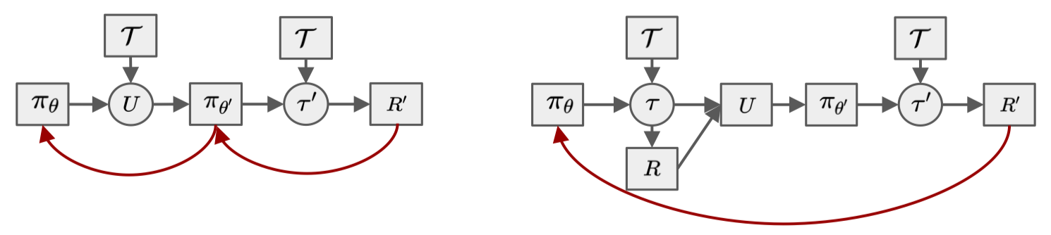
This figure also illustrates the change of relation between \(U\) and \((\mathcal T,\pi_\theta)\). In formulation \(I\), \(U\) is a function directly depending on \((\mathcal T,\pi_\theta)\) through \(P_{\mathcal T}(\tau\vert \theta)\). In contrast, formulation \(II\) samples \(\tau\) from \(P_{\mathcal T}(\tau\vert \theta)\) first, then constructs \(U\) from \(\tau\), breaking the direct dependence between \(U\) and \((\mathcal T, \pi_\theta)\). We refer readers unfamiliar with stochastic computation graphs to our previous post.
Terms in Gradients
In this section, we further study each terms in formulations \(I\) and \(II\). First, we rewrite them as follows
\[\begin{align} {\nabla_\theta J_{post}(\tau,\tau')}&=\big(I+R(\tau)\alpha\nabla_\theta^2\log\pi_{\theta}(\tau)\big)\nabla_{\theta'}\log\pi_\theta(\tau')R(\tau')\\\ {\nabla_\theta J^I_{pre}(\tau,\tau')} &=\alpha\nabla_\theta\log\pi_\theta(\tau)\Big(\underbrace{(\nabla_\theta\log\pi_\theta R(\tau))^T}_{\nabla_\theta J^{inner}}\underbrace{(\nabla_{\theta'}\log\pi_{\theta'}(\tau')R(\tau')}_{\nabla_{\theta'} J^{outer}})\Big)\\\ {\nabla_\theta J^{II}_{pre}(\tau,\tau')}&=\alpha\nabla_\theta\log\pi_\theta(\tau)R(\tau') \end{align}\]Taking a closer look at each term, we can see
-
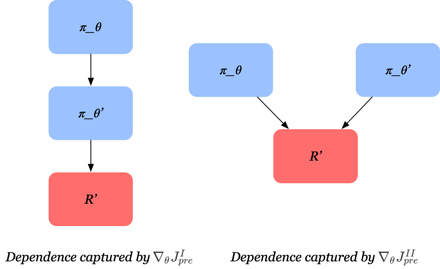
\(\nabla_\theta J_{post}(\tau,\tau’)\) is equal in both formulas. It simply corresponds to a policy gradient step on the post-update policy \(\pi_{\theta’}\) w.r.t. \(\theta’\), followed by a linear transformation from post- (\(\theta’\)) to pre-update parameters (\(\theta\)). This term increases the likelihood of the trajectories \(\tau’\) that lead to higher returns, but it does not optimize for the pre-update sampling distribution, i.e., which trajectory \(\tau\) leads to better adaptation steps.
-
The credit assignment w.r.t. the pre-updated sampling distribution is carried out by the second term. \(\nabla_\theta J_{pre}^{II}\) can be viewed as standard policy gradient on \(\pi_\theta\) with \(R(\tau’)\) as reward signal, treating the update function \(U\) as part of the unknown dynamics of the system. This shifts the pre-update sampling distribution so that higher post-update returns are achieved. However, this term omits the causal dependence of the post-update policy on the pre-update policy. This implies that increasing the impact of \(\pi_\theta\) on \(R’\) may weaken that of \(\pi_{\theta’}\) on \(R’\). The figure above demonstrates this difference.
-
Formulation \(I\) takes the causal dependence of \(P_{\mathcal T}(\tau’\vert \theta’)\) on \(P_{\mathcal T}(\tau\vert \theta)\) into account. It does so by maximizing the inner product of pre-update and post-update policy gradient (see \(\nabla_\theta J_{pre}^I\)). This steers the pre-update policy towards 1) larger post-update returns(i.e., larger \(R(\tau’)\)) 2) larger adaptation steps(i.e., larger \(\pi_{\theta’}\)) 3) better alignment of pre- and post-update policy gradients (i.e., larger \((\nabla_\theta\log\pi_\theta)^T\nabla_{\theta’}\log\pi_{\theta’}\))
ProMP: Proximal Meta-Policy Search
In this section, we briefly discuss the potential problem of the original implementation of MAML-RL, and introduce ProMP, proposed by Rothfuss, Lee&Clavera et al., to address the issue. As for the detailed reasoning, please refer to the original paper; I’m going to take a rain check, J.
Low Variance Curvature Estimator
Although MAML-RL proposed by Finn et al. is theoretically sound, the corresponding implementation neglects \(\nabla_\theta J^I_{pre}\), resulting in highly biased estimate. To address this issue, Rothfuss, Lee&Clavera et al. introduce the low variance curvature(LVC) estimator:
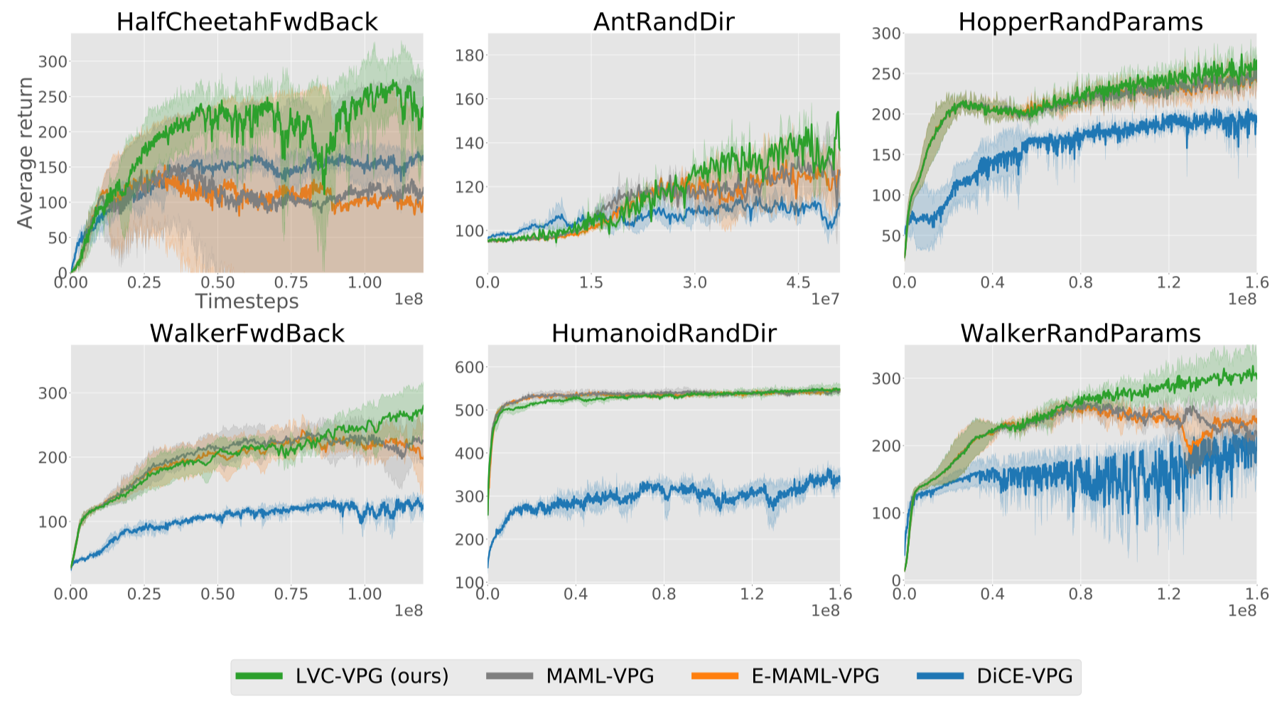
\[\begin{align} J^{LVC}(\tau)=\sum_{t=0}^{H-1}{\pi_\theta(a_t|s_t)\over\perp(\pi_\theta(a_t|s_t))}\left(\sum_{t'=t}^{H-1}r(s_{t'},a_{t'})\right) \end{align}\]where \(\perp\) denotes the “stop_gradient” operator. The second derivative of this estimator has lower variance than DiCE, proposed by Foerster et al[5], but makes the estimate biased. This bias of LVC estimator, under some conditions, becomes negligible close to local optima. The following figure shows LVC estimator experimentally improves the sample-efficiency of meta-learning by a significant margin compared to DiCE
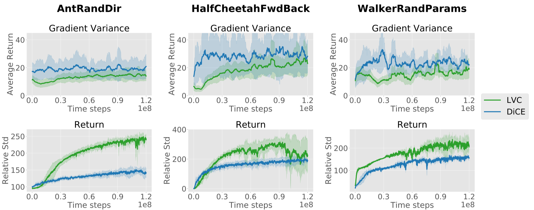
The \(y\) axes are mislabeled in the above figure. The graphs on the top have standard deviation as \(y\)-axis, while the graphs on the bottom have average return as \(y\)-axis.
ProMP
ProMP uses PPO to ease the computational cost of TRPO. In particular, it defines post-update objective as follows
\[\begin{align} J^{ProMP}_{\mathcal T}(\theta)&=J_{\mathcal T}^{CLIP}(\theta')-\eta D_{KL}(\pi_{\theta_{o}},\pi_\theta)\\\ J_{\mathcal T}^{CLIP}&=\mathbb E_{\tau\sim P_{\mathcal T}(\tau|\theta)}\left[\sum_{t=0}^{H-1}\min \left({\pi_\theta(a_t|s_t)\over\pi_{\theta_{o}(a_t|s_t)}}\hat A_t, \mathrm{clip}\left({\pi_\theta(a_t|s_t)\over\pi_{\theta_{o}(a_t|s_t)}}, 1-\epsilon, 1+\epsilon\right)\hat A_t\right)\right] \end{align}\]where \(\pi_{\theta_o}\) is the original policy, which we do not compute gradient through, and \(\eta=0.005\). The author further introduce the KL term in additional to the original PPO objective to bound changes in the pre-update state visitation distribution.
The pre-update objective modifies the LCV estimator a bit to account for changes in the pre-update action distribution \(\pi_\theta(a_t\vert s_t)\)
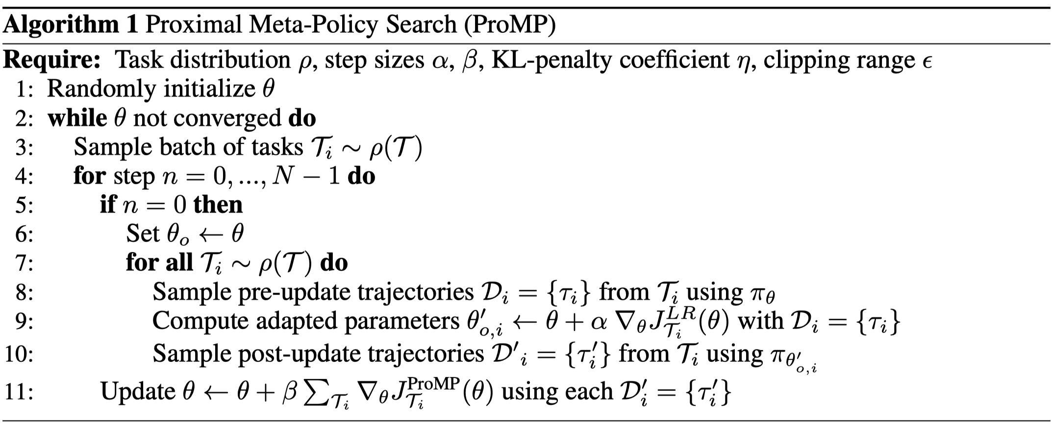
\[\begin{align} J^{LR}_{\mathcal T}(\theta)=\mathbb E_{\tau\sim P_{\mathcal T}(\tau,\theta_o)}\left[\sum_{t=0}^{H-1}{\pi_\theta(a_t|s_t)\over\pi_{\theta_o}(a_t|s_t)}A^{\pi_{\theta_o}}(s_t,a_t)\right] \end{align}\]The entire algorithm is described as follows
Experimental Results
We present experimental results across six different locomotion tasks
References
- Jonas Rothfuss, Dennis Lee, Ignasi Clavera, Tamim Asfour, Pieter Abbeel ProMP: Proximal Meta-Policy Search. In ICLR 2019
- Chelsea Finn, Pieter Abbeel, Sergey Levine. Model-Agnostic Meta-Learning for Fast Adaptation of Deep Networks
- Maruan Al-Shedivat, Trapit Bansal, Umass Amherst, Yura Burda, Openai Ilya, Sutskever Openai, Igor Mordatch Openai, and Pieter Abbeel. Continuous Adaptation via Meta-Learning in Nonstationary and Competitive Environments. In ICLR 2018
- Bradly C. Stadie, Ge Yang, Rein Houthooft, Xi Chen, Yan Duan, Yuhuai Wu, Pieter Abbeel, Ilya Sutskever. Some Considerations on Learning to Explore via Meta-Reinforcement Learning
- Jakob Foerster, Gregory Farquhar, Maruan Al-Shedivat, Tim Rocktaschel, Eric P Xing, and Shimon Whiteson. DiCE: The Infinitely Differentiable Monte Carlo Estimator. In ICML, 2018.