
Introduction
Exploration plays an important role in reinforcement learning: it helps agents to explore the environment, and therefore learn potential better policy. In this post, we discuss a set of active exploration methods, involving exploration bonus, Thompson sampling, and information gain exploration. For every strategy, we will first present some intuition and their uses in multi-bandit environment, in which we have \(N\) action choices \({a_1,\dots,a_N}\), and each action \(a_i\) yields a reward \(r(a_i)\) sampled from an unknown distribution \(p_i(r(a_i))\). Then we bring them to the Markov decision process, introducing some algorithms built upon these theories.
Exploration Bonus
Exploration Bonus in Multi-Bandit
In exploration bonus(aka. optimistic exploration), we keep track of average reward \(\hat \mu_a\) for each action \(a\), and we take into account our confidence of uncertainty when we choose an action:
\[\begin{align} a=\arg\max_a\hat \mu_a+C\sigma_a\tag {1} \end{align}\]where \(C\) is a hyperparameter and \(\sigma_a\) is a variance estimate of uncertainty that becomes smaller as the action \(a\) is taken more often. The intuition behind this is: if some action is taken rarely, we tend to optimistically think it might have a high reward. As the action is taken, we increase our confidence in the action and tend to regard the average reward as the expected reward of taking the action. An example is Upper Confidence Bound(UCB), which defines \(\sigma_a\) as
\[\begin{align} \sigma_a=\sqrt{2\log t\over N(a)} \end{align}\]where \(t\) counts the total actions taken and \(N(a)\) is the times action \(a\) is taken. In practice, a simpler \(\sigma_a\) could also work
\[\begin{align} \sigma_a=\sqrt{1\over N(a)}\tag {2} \end{align}\]Exploration Bonus in Markov Decision Process
Exploration bonus in multi-bandit optimistically gives a high exploration bonus \(C\sigma_a\) to actions rarely tried. Applying this idea to an MDP, we could optimistically gives a high reward to new states(or new state-action pairs). In high-dimensional problems or continuous problems, this requires a way of estimating the novelty measure that tells us how novel a state is since states are rarely revisited in those problems.
In count-based methods, novelty is measured by a pseudo count \(\hat N(s)\), analogous to \(N(a)\) in Eq.\((2)\)(although \(\hat N(s,a)\) is more sensible for action selection, for the sake of simplicity, we still consider \(\hat N(s)\) in the following discussion). There are many choices explored in literature, here we only introduce several of them mentioned by Sergey Levine in his class:
Unifying Count-Based Exploration and Intrinsic Motivation
Assume we have the state distribution model \(p_\theta(s)\). For each state \(s\) the agent observes, we have two state distribution models: one trained before observing \(s\), \(p_\theta(s)\), and the other refitted after observing \(s \), \(p_{\theta’}(s)\). Then we solve the following two equations to obtain \(\hat N(s)\).
\[\begin{align} p_\theta(s)&={\hat N(s)\over \hat n}\\\ p_{\theta'}(s)&={\hat N(s)+1\over \hat n+1} \end{align}\]Now we come back to \(p_\theta(s)\), Bellemare et al. proposes a “CTS” model, which approximate \(p_\theta(s)\) using
\[\begin{align} p_\theta(s)=\prod_{i,j}p_{\theta_{i,j}}(x^{i,j}|x^{i-1,j},x^{i,j-1},x^{i-1,j-1},x^{i-1,j+1}) \end{align}\]where \(x^{i,j}\) is a pixel located at position \((i,j)\), the and \(p_{\theta_{i,j}}\) may be a network that takes as input the top-left neighbourhood of \(x^{i,j}\) and outputs the probability of \(x^{i,j}\) (which is only my conjecture. I have not gone into detail of the paper.)
Exploration: A Study of Count-Based Exploration
In this method, we compute the pseudo count following three steps:
- Representation Learning: Compress the state to obtain a brief representation \(g(s)\) using some pre-trained model
- Locality-Sensitive Hashing: Hash the representation into a \(k\)-bit code \(\phi(g(s))\)
- Occurrence Counting: Update the occurrence of the \(k\)-bit code \(N(\phi(g(s)))=N(\phi(g(s)))+1\)
The first step could be achieved by some representation learning algorithm, such as autoencoder. A computationally efficient type of locality-sensitive hashing(LSH) is SimHash, which measures similarity by angular distance. SimHash retrieves a binary code of state \(s\) as
\[\begin{align} \phi(s)=\mathrm{sgn}(Ag(s))\in\{-1, 1\}^k \end{align}\]where \(A\) is a \(k\times D\) matrix with i.i.d. entries draw from a standard Gaussian distribution \(\mathcal N(0, 1)\). The value of \(k\) controls the granularity; higher values lead to fewer collisions and are thus more likely to distinguish states.
EX\(^2\): Exploration with Exemplar Models for Deep Reinforcement Learning
EX\(^2\) does not explicitly compute the pseudo count. Instead, it computes the probability density of state \(p(s)\) through a discriminator that distinguishes the new state(exemplar) from all the previous states. Such a discriminator has a binary cross entropy loss
\[\begin{align} \mathcal L(D)=-\mathbb E_{\delta_{s^\*}}[\log D(s)]-\mathbb E_{p(s)}[\log (1-D(s))] \end{align}\]where \(s^*\) is the new state, \(\delta_{s^*}\) is a delta distribution centered at \(s^*\), and \(p(s)\) is the previous state distribution. When the discriminator is optimal, the gradient of the loss w.r.t. \(D(s^*)\) is zero:
\[\begin{align} \nabla_{D(s^\*)}\mathcal L(s)=-{1\over D(s^\*)}+{p(s^\*)\over 1-D(s^\*)}=0 \end{align}\]solving the equation, we have
\[\begin{align} p(s^\*)={1-D(s^\*)\over D(s^\*)} \end{align}\]Then we employ \(-\log p(s)\) as the exploration bonus instead of Eq.\((2)\) used before.
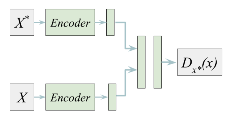
The above discriminator is kind of specialized to a single exemplar, and therefore we have to train a discriminator for each new state. This is impractical in practice, and we could unify all discriminators by conditioning a single discriminator on the exemplar. The resulting architecture is shown on the right, where \(X^*\) is the exemplar and \(X\) is the input data for the discriminator to distinguish (where the exemplar is labeled positive and the others are labeled negative). In practice, we use the same amount of positive and negative data for fair training.
As a last note, the authors of the paper propose using a VAE structure to further introduce disentanglement for state generalization. The resulting objective is almost the same as that of VAE except that we do classification at the end rather than reconstructing the data.
The resulting algorithm works as follows
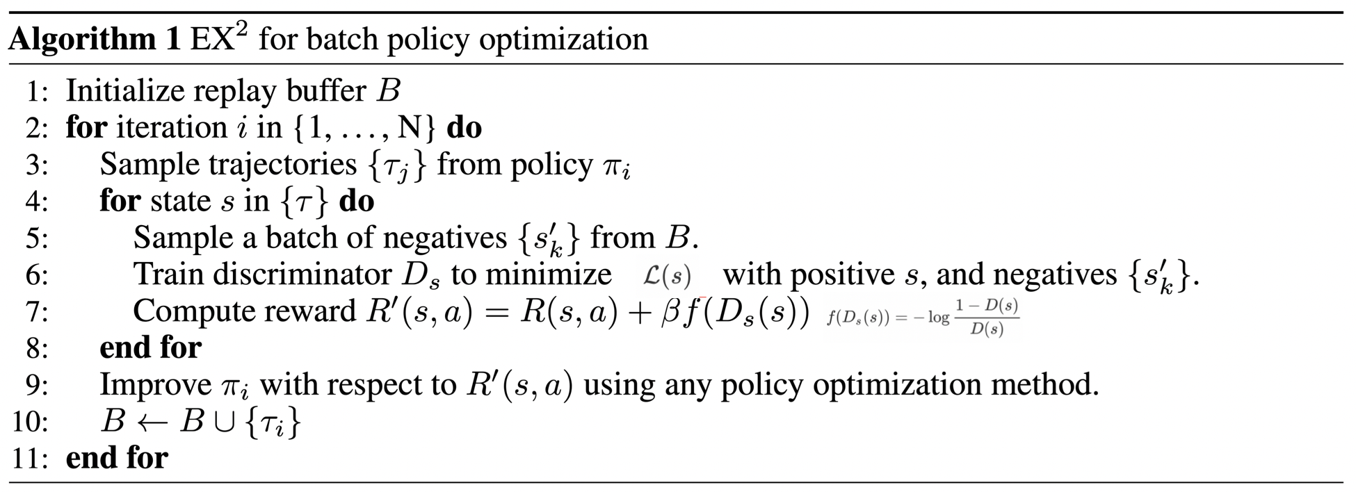
I personally think it may be better for on-policy RL methods to trains the discrimiantor several steps first after sampling and then compute rewards without further training the discriminator.
Thompson Sampling
Thompson Sampling in Multi-Bandit
For each arm \(a_i\), we parameterize the reward distribution by \(\theta_i\). Since we don’t know the reward distribution beforehand, we maintain a belief about the parameters \(\theta_i\). Let \(p(\theta_i)\) be the belief distribution of \(\theta_i\). Then, for every arm, we play it with the probability of it being the best. Let’s say we play arm \(a_i\) and receive reward \(r_i\). After that, we update our belief about the reward distribution of arm \(a_i\) using Bayes’ rule: \(p(\theta_i\vert r)\propto p(\theta_i)p(r\vert \theta_i)\). We take \(p(\theta_i\vert r)\) as our new belief distribution of \(\theta_i\) and repeat the above process until convergence. A concise algorithm description is given as below
\[\begin{align} &1.\quad\mathrm{Initialize\ prior\ parameter\ distributions\ }p(\theta_1),\dots, p(\theta_n)\\\ &2.\quad\mathrm{For\ }t=1,\dots:\\\ &3.\quad\quad \mathrm{Sample\ }\hat\theta_1,\dots, \hat\theta_n\sim p(\theta_1),\dots, p(\theta_n)\\\ &4.\quad\quad \mathrm{Take\ the\ optimal\ action\ }a_i\ \mathrm{w.r.t.\ }\hat\theta_1,\dots,\hat\theta_n\\\ &5.\quad\quad \mathrm{Observe\ reward\ }r\ \mathrm{and\ update\ posterior}\ p(\theta_i)\propto p(\theta_i)p(r|\theta_i) \end{align}\]Thompson Sampling in Markov Decision Process
In order to transfer Thompson sampling to MDP, we could simultaneously learn multiple \(Q\)-functions or policies (in contrast to the reward distribution). Then, at every step, we sample a \(Q\)-function(or policy) and act according to the sample. In practice, we could share most of the layers (except the last one) of the \(Q\)-functions(policies) to gain some additional efficiency.
A simpler approach is noisy networks, a special form of Bayesian neural networks(which will be further elaborated in the next section) where weights are of Gaussian distributions.
Information Gain Exploration
Information gain exploration is similar to exploration bonus in that both values new states optimistically by adding an extra bonus to the reward. The difference is that information gain exploration explicitly reasons about how much the agent will learn from visiting new states, rather than simply assuming that something is good because it is new.
Variational Information Maximizing Exploration
One way to apply information gain to MDP, is to consider the reduction in uncertainty about the dynamics as information gain. The intuition is that we prefer to explore states where we can learn more about the dynamics. Variational Information Maximizing Exploration(VIME) formulates the above intuition as maximizing the conditional information gain of the dynamics model parameter \(\Theta\) from the next state \(S_{t+1}\).
\[\begin{align} I(\Theta; S_{t+1}|h_t, a_t)&=D_{KL}[p(\theta,s_{t+1}|h_t,a_t)\Vert p(\theta|h_t)p(s_{t+1}|h_t,a_t)]\\\ &=\mathbb E_{s_{t+1}\sim p(\cdot|h_t,a_t)}[D_{KL}[p(\theta|h_t,a_t,s_{t+1})\Vert p(\theta|h_t)]]\tag {3} \end{align}\]where \(h_t\) is a history of states and actions up to time step \(t\), and \(s\) and \(a\) denote the state and action as usual. Once we obtain this information gain, we can add it to the reward to achieve the trade-off between exploitation and exploration
\[\begin{align} r'(s_t, a_t, s_{t+1})=r(s_t,a_t)+\eta D_{KL}[p(\theta|h_t,a_t,s_{t+1})\Vert p(\theta|h_t)] \end{align}\]In the above reasoning, the parameter is stochastic, which provides a way of measuring the uncertainty about the model. This, however, forbids us from using general neural networks, of which parameters are deterministically learned by maximum likelihood estimation (or maximum a posteriori if regularization is involved). That’s where Bayesian neural networks(BNNs) come into play. In BNNs, parameters are, just as we expect, sampled from distributions and the inference are made through the integral
\[\begin{align} p(y|x)&=\int p(y|x,\theta)p(\theta|\mathcal D)d\theta\\\ where\quad p(\theta|\mathcal D)&={p(\mathcal D|\theta)p(\theta)\over\int p(\mathcal D|\theta)p(\theta)d\theta} \end{align}\]However, the above equation cannot be solved as we do with general neural network since it involves integral over the parameter space. Fortunately, our objective here is to learn the parameter distributions instead of dong inference. In order to learn the posterior distribution \(p(\theta\vert \mathcal D)\), we could resort to variational inference, where we approximate \(p(\theta\vert \mathcal D)\) using an alternative distribution \(q(\theta\vert \phi)\), which is optimized through maximization of the evidence lower bound(ELBO):
\[\begin{align} \mathbb E_{q(\theta|\phi)}[\log p(\mathcal D|\theta)]-D_{KL}[q(\theta|\phi)\Vert p(\theta)]\tag {4} \end{align}\]where \(\phi\) could be the mean and variance of each parameter if we take the variational posterior as a diagonal Gaussian distribution.
Now that we have parameterized the dynamics model parameter \(\theta\) by \(\phi\), we express the information gain as the KL divergence between the variational models after and before observing the next state as Eq.\((3)\) suggested
\[\begin{align} I(\theta|\phi; s_{t+1})&=D_{KL}[q(\theta|\phi_{t+1})\Vert q(\theta|\phi_t)]\tag {5} \end{align}\]where \(\phi_{t+1}\) and \(\phi_t\) are the updated and the old parameters, respectively. To compute the updated parameter \(\phi_{t+1}\), we minimize
\[\begin{align} D_{KL}[q(\theta|\phi)\Vert q(\theta|\phi_{t})]-\mathbb E_{q(\theta|\phi)}[\log p(s_{t+1}|h_t,a_t,\theta)]\tag {6} \end{align}\]which could be roughly regarded as the negative of the ELBO w.r.t. the single transition the agent just experienced. In practice, Houthooft et al. propose to efficiently optimize Eq.\((6)\) through Newton’s method. Because it’s more like an implementation details, we refer to interested readers to Eq.\((13)\)-Eq.\((16)\) in the paper.
So far we have introduced two evidence lower bounds: Eq.\((4)\) and Eq.\((6)\). Although both optimize \(q(\theta\vert \phi)\), they serve different purposes. Eq.\((4) \) globally updates the variational model \(q(\theta\vert \phi)\) to approximate \(p(\theta\vert \mathcal D)\), Eq.\((6)\) temporarily computes \(q(\theta\vert \phi_{t+1})\) to obtain the information gain from \(s_{t+1}\), and is discarded afterwards.
Algorithm
Well, the above presentation might be a little chaotic :-(. Let us sum it up.
The algorithm repeats the following steps:
\[\begin{align} 1.\quad& \mathrm{For\ }t=1\dots,T:\\\ 2.\quad&\quad\mathrm{Run\ the\ policy}\ \pi\ \mathrm{to\ collect\ transition}\ (s_t,a_t,s_{t+1})\mathrm{\ and\ reward\ }r(s_t,a_T),\\\ &\quad\mathrm{adding\ transition\ to\ replay\ buffer}\\\ 3.\quad&\quad\mathrm{Compute\ information\ gain\ }I(\theta|\phi; s_{t+1})\\\ 4.\quad&\quad \mathrm{Construct\ new\ reward\ }r'(s_t, a_t, s_{t+1})=r(s_t,a_t)+\eta I(\theta|\phi;s_{t+1})\\\ 5.\quad&\mathrm{Optimize\ Eq.(3)\ to\ update\ }q(\theta|\phi)\mathrm{\ with\ data\ sampled\ from\ replay\ buffer}\\\ 6.\quad&\mathrm{Use\ rewards\ }\{r'(s_t,a_t,s_{t+1})\}\mathrm{\ to\ update\ policy\ \pi\ using\ some\ model-free\ method} \end{align}\]Instead of using the KL divergence in Eq.\((5)\) directly as an intrinsic reward, Houthooft et al. propose to normalize it by division through the average of the median KL divergences taken over a fixed number of previous trajectories. Doing so, we emphasizes relative difference in KL divergence between samples, rather than focusing on its absolute value.
Recap
In this post, we’ve briefly introduced three types of exploration strategy in reinforcement learning.
Perhaps the most fundamental strategy is exploration bonus, and we’ve discussed three related algorithms: The first counts the new state by solving \(p_\theta(s)={\hat N(s)\over \hat n}\) and \(p_{\theta’}(s)={\hat N(s)+1\over \hat n+1}\) where \(p_\theta(s)\) is computed via a “CTS” model; The second hashes the encoded new state into a \(k\)-bit code and counts the \(k\)-bit code; The last measures how novel the new state is using a discriminator, which distinguishes the new state from all previous states. Unlike the previous two methods, which computes the exploration bonus via a pseudo-count, the last method takes \(-\log p(s)\) as the exploration bonus instead.
Then we talked about Thompson sampling, which maintains a belief of the target (e.g. \(Q\)-functions and policies). In Thompson sampling, we make an action based on a random sample from the belief. One simple example is noisy networks, an algorithm we’ve seen back the day when we talked about Rainbow.
The last strategy is about information gain, which directly reasons about how much we will learn from the new state. And we have seen VIME utilizes variational inference to approximate dynamics model and take the KL divergence between the variational models after and before observing the new state as information gain.
Reference
CS 294-112 at UC Berkeley. Deep Reinforcement Learning Lecture 16
Marc G. Bellemare et al. Unifying Count-Based Exploration and Intrinsic Motivation
Haoran Tang et al. Exploration: A Study of Count-Based Exploration for Deep Reinforcement Learning
Justin Fu et al. EX\(^2\) : Exploration with Exemplar Models for Deep Reinforcement Learning
Charles Blundell et al. Weight Uncertainty in Neural Networks
Rein Houthooft et al. VIME: Variational Information Maximizing Exploration