
Contrastive Predictive Coding
Overview
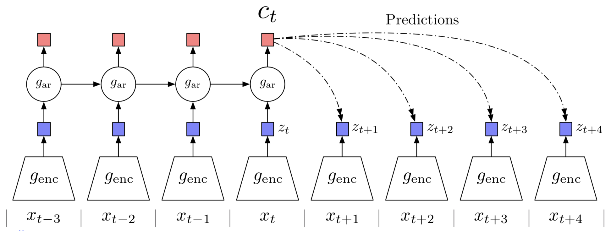
Contrastive Predictive Coding(CPC) tries to learn the “slow representation” that encode the underlying shared information spanning many time steps. At the same time it discards low-level information and noise that is more local. As a result, CPC encodes the target \(x\) and maximizes the mutual information between the encoded representation \(z\) with the context \(c\). This gives us the structure shown in the above figure, which mainly consists of three parts:
- An encoder, which compresses high-dimensional data \( x_t \) into a more compact latent vectors \( z_t \) in which conditional predictions are easier to model
- An autoregressive model, which further distills a context representation \( c_t \) shared across the encoded latent vectors in the previous timestamps (\( \dots, z_{t-2}, z_{t-1} \))
- A set of networks (each for a prediction) or simply an autoregressive model used for ‘predictions’. That is, we expect to use \( f_k(c_t) \) to resemble \( z_{t+k} \), where \( f_k \) is represented by a neural network.
Long story short, the first two parts distill the high-level information \( c_t \) that spans many steps, while the third part compares the predictions with their corresponding \( z_{t+k} \) to adjust all three networks.
Now let’s take a deeper look at each part.
Encoding Observations
The encoder could be any architecture that takes as input an observation \( x \) outputs a concise, high-level representation \( z \). One of the reasons why we encode all data in time series is to avoid the networks in the prediction stage trying to reconstruct every detail in the data. Such reconstructions always result in powerful generative models, which are computationally intense, and waste the capacity at modeling the complex relationships in the data, often ignoring the context \( c \) distilled in the second stage.
Summarizing History
An autoregressive model (such as RNN-variant architectures, temporal convolution networks, or self-attention networks) summarizes all previous latent representations \( z_{\le t} \) and produces a context latent representation \( c_t \). This context representation encodes the sequential information from the latent representation \( z_{\le t} \) and is capable of conjecture the future.
Predicting Future
Any model, mapping \( c_t \) to \( z_{t+k} \) where \( k>0 \), can be used in this stage. However, raw predictions could be redundant even in latent space. The authors instead propose modeling a density ratio which preserves the mutual information between \(x_{t+k}\) and \(c_t\) as follows(see discussion in the next sub-section for details):
\[\begin{align} f_k(x_{t+k},c_t)\propto{p(x_{t+k}|c_t)\over p(x_{t+k})}\tag{1} \end{align}\]Although any positive real score can be used here, we use a simple log-bilinear model
\[\begin{align} f_k(x_{t+k}, c_t)=\exp(z_{t+k}^TW_kc_t) \end{align}\]where we use one perception \(W_kc_t\) for each \(z_{t+k}\). Alternatively, more complicated models such as recurrent neural networks also could be used.
One thing may be worth keeping in mind: The prime thing we do here is not prediction, our objective is to maximize the mutual information between \( c_t \) and \( x_{t+k} \) so as to improve our model.
Loss
All network are trained to jointly optimize a loss based on Noise Contrastive Estimation loss(NCE), which we call InfoNCE. Given a set \(X={x^1,\dots, x^N}\) of \(N\) random samples containing one positive sample from \(p(x_{t+k}\vert c_t)\) and \(N-1\) negative samples from the ‘proposed’ distribution \(p(x_{t+k})\), the InfoNCE is defined as:
\[\begin{align} L=-E_X[\log p(d=i|X,c_t)]=-\mathbb E_X\left[\log{f_k(x_{t+k}, c_t)\over \sum_{x_j\in X}f_k(x_j, c_t)}\right]\tag{2} \end{align}\]where \(p(d=i\vert X,c_t)\) is the probability with \([d=i]\) being the indicator that sample \(x^i\) is the ‘positive’ sample drawn from \(p(x_{t+k}\vert c_t)\). The optimal probability for this loss is
\[\begin{align} p(d=i|X,c_t)&={p(d=i,X|c_t)\over\sum_{j=1}^Np(d=j, X|c_t)}\\\ &={p(x^i|c_t)\prod_{l\ne i}p(x^l)\over\sum_{j=1}^Np(x^j|c_t)\prod_{l\ne j}p(x^l)}\\\ &={ {p(x^i|c_t)\over p(x^i)}\over\sum_{j=1}^N{p(x^j|c_t)\over p(x^j)}} \end{align}\]As we can see, the optimal value for \(f(x_{t+k}, c_t)\) in Eq.2 is proportional to \(p(x_{t+k}\vert c_t)\over p(x_{t+k})\) and is independent of the choice of the number of negative samples \(N-1\).
We can also prove that minimizing Equation 2 is equivalent to maximizing the mutual information between \(c_t\) and \(x_t\):
\[\begin{align} L&=-\mathbb E_X\left[\log { {p(x_{t+k}|c_t)\over p(x_{t+k})}\over {p(x_{t+k}|c_t)\over p(x_{t+k})}+ \sum_{x_j\in X_{neg}}{p(x_{j}|c_t)\over p(x_j)} }\right]\\\ &=\mathbb E_X\log\left[1+{p(x_{t+k})\over p(x_{t+k}|c_t)}{\sum_{x_j\in X_{neg}}{p(x_{j}|c_t)\over p(x_{j})}}\right]\\\ &\approx\mathbb E_X\log\left[1+{p(x_{t+k})\over p(x_{t+k}|c_t)}(N-1)\mathbb E_{x_j}{p(x_{j}|c_t)\over p(x_{j})}\right]\\\ &=\mathbb E_X\log\left[1+{p(x_{t+k})\over p(x_{t+k}|c_t)}(N-1)\right]\\\ &\ge\mathbb E_X\log\left[{p(x_{t+k})\over p(x_{t+k}|c_t)}N\right]\\\ &=-I(x_{t+k},c_t)+\log N \end{align}\]CPC with Images
When applying CPC to images, we divide the image into several patches. The prediction task becomes to predict a the representations of pathces below a certain position from those above it. In practice, the context network that summarizes the past is a 1D masked convolutional network, where the masks are such that the receptive field of each resulting context vector \(c_{i,j}\) only includes feature vectors that lie above it in the image.
CPCv2
Hénaff et al. 2020 improves cpc with the following modifications:
- They use a larger network and large input patch size
- They use layer normalization instead of batch normalization. They actually find batch normalization impairs the downstream perfomance. They hypothesize that batch normalization introduces a dependency between patches (through the batch statistics) and can be exploited to bypass the constraints on the receptive field.
- In addition to predict each patch only context from the above, they also predict the same patch using context from below, the right and the left (using separate context networks).
- They employ color dropping which randomly drops two of the three color channels in each patch, as well as random horizontal flips.
Interaction with Reinforcement Learning
It might be helpful to use the context \( c_t \) as the input state to reinforcement learning algorithms, which helps the agent to think beyond the Markov property. That is, the agent may now make decisions based not only on the current state, but also on the summarized information from the past and prediction of the future.
Supplementary Materials
A function \(f\) is symmetric bilinear if it sastisfies the following properties
- \(f(u,v)=f(v,u)\)
- \(f(\alpha u,v)=f(u,\alpha v)=\alpha f(u,v)\),
- \(f(u+v,w)=f(u,w)+f(v,w)\)
- \(f(u,v+w)=f(u,v)+f(u,w)\)
The first is symmetric, the rest are bilinear.
References
Oord, Aaron van den, Yazhe Li, and Oriol Vinyals. 2018. “Representation Learning with Contrastive Predictive Coding.” http://arxiv.org/abs/1807.03748.
Hénaff, Olivier J., Aravind Srinivas, Jeffrey De Fauw, Ali Razavi, Carl Doersch, S. M. Ali Eslami, and Aaron van den Oord. 2019. “Data-Efficient Image Recognition with Contrastive Predictive Coding.” http://arxiv.org/abs/1905.09272.