
Introduction
Although model-free algorithms have shown great potential in solving many challenging tasks, such as Atari and StarCraft, they are still far from the state of the art in domains that requires precision and sophisticated lookahead, such as chess and Go. On the other hand, planning algorithms are able to master chess and Go but they usually rely on the knowledge of the environment’s dynamics, preventing their application to real-world domains like robotics. We discuss a model-based RL agent named MuZero, the successor of AlphaZero also proposed by Silver et al. 2019 at DeepMind, that achieves state-of-the-art performance in Atari 2600 while maintaining superhuman performance in precision planning tasks.
Notice that throughout this post, we associate \(a_{t+1}\) and \(r_{t+1}\) with \(s_t\) following the convention adopted by the paper.
TL; DR
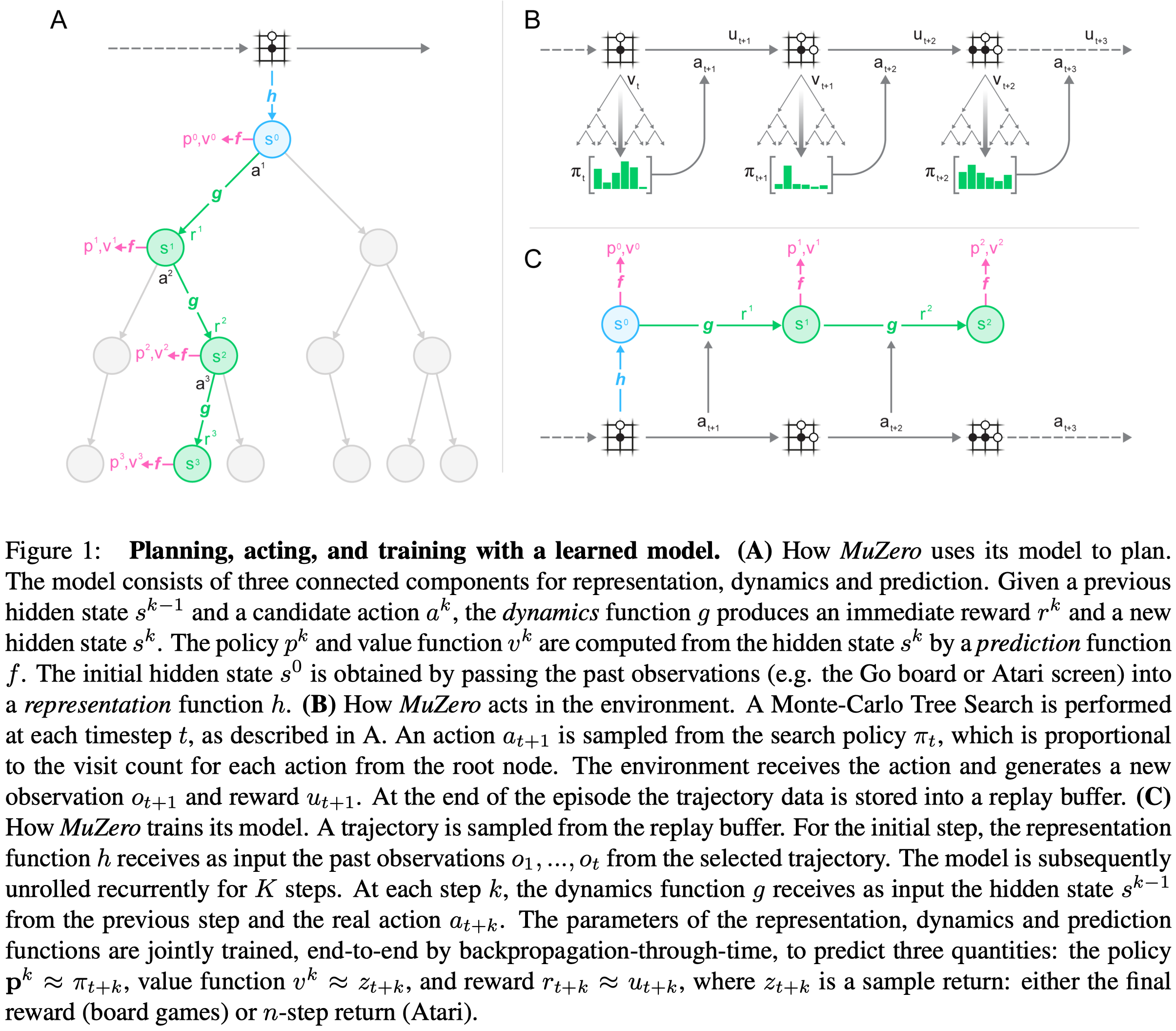
MuZero, the successor of AlphaZero, dispenses with the simulator and trains a representation model and a dynamics model to learn the hidden dynamics. Both the representation and the dynamics models are deep ResNets. The representation model maps the a history of observations to a latent space, from which the dynamics model predict the immediate reward and the next state. Mathematically, we have
\[\begin{align} \text{representation model:}&&s^0=&h_\theta(o_1,\dots,o_t)\\\ \text{dynamics model:}&&r^k,s^k=&g_\theta(s^{k-1},a^k)\\\ \text{AC model:}&&p^k,v^k=&f_\theta(s^k) \end{align}\]Notice that MuZero assumes deterministic transition dynamics.
During training, MuZero unrolls the network for \(K=5\) hypothetical steps. To maintain a roughly similar magnitude of gradient across different unroll steps, we 1) scale the loss of each head by \(1\over K\) and 2) scale the gradient at the start of the dynamics function by \(1/2\). Moreover, the hidden state are scaled to the same range as the action: \(s_{scale}={s-\min(s)\over\max(s)-\min(s)}\).
For Atari, the value function is updated with \(n=10\)-step bootstrapped target.
Table of Contents
This post is comprised of the following components
Inference
Similar to AlphaZero, MuZero is based upon Monte-Carlo Tree Search(MCTS) with upper confidence bounds(UCB). Every node in the search tree is associated with an internal state \(s\). For each action \(a\) from \(s\) there is an edge \((s,a)\) that stores a set of statistics \({N(s,a), Q(s,a), P(s,a), R(s,a),S(s,a)}\), respectively representing visit counts \(N\), mean action value \(Q\), policy \(P\), reward \(R\), and state transition \(S\). Here, we represent the dynamics function deterministically; the extension to stochastic transitions is still left for future work. The start state \(s^0\) is obtained through a representation function \(h\), which encodes the input planes into an initial state \(s^0\) (Figure 1).
The search repeats the following three stages for \(N\) simulations(\(N=800\) for board games and \(N=50\) for Atari):
Selection
Each simulation starts from the internal root state \(s^0\) and finishes when the simulation reaches a leaf node \(s^l\). For each step \(k=1,\dots,l\) in the search tree, an action \(a^{k}\) is selected to maximize over a variant of upper confidence bound(UCB), the same one defined in AlphaZero
\[\begin{align} a^{k}=\underset a{\arg\max}\left[Q(s,a)+P(s,a)\cdot{\sqrt{\sum_bN(s,b)}\over1+N(s,a)}\left(c_1+\log\left({\sum_b N(s,b)+c_2+1\over c_2}\right)\right)\right]\tag{1} \end{align}\]where \(c_1\) and \(c_2\) control the influence of the prior policy \(P(s,a)\) relative to the value \(Q(s,a)\) as nodes are visited more often. In their experiments \(c_1=1.25\) and \(c_2=19652\)…
For \(k< l\), rewards and next states are looked up in the state transition and reward table \(s^k=S(s^{k-1}, a^k)\), \(r^k=R(s^{k-1},a^k)\).
For board game, Dirichlet exploration noise is applied to the root of the search tree as in AlphaZero.
Expansion
At the final time-step \(l\), where we expand a new node \(s^l\), the reward and next state are computed by the dynamics function, \(r^{l},s^{l}=g(s^{l-1},a^{l})\), and stored in the corresponding tables \(R(s^{l-1}, a^{l})=r^{l},S(s^{l-1},a^{l})=s^{l}\). The new node, corresponding to state \(s^l\), is added to the search tree, and the policy and value are computed by the prediction function, \(\pmb p^l,v^l=f(s^l)\). Each edge \((s^l,a)\) from the newly expanded node is initialized to \({N(s^l,a)=0,Q(s^l,a)=0,P(s^l,a)=\pmb p^l}\). Note that the search algorithm makes at most one call to the dynamics function \(g\) and prediction function \(f\) respectively per simulation and the statistics of edges from the newly expanded node are not updated at this point. As a concrete example, consider Figure 1a. At time step \(3\), MCTS expands \(s^3\) and compute \(g(s^2,a^3)\) and \(f(s^3)\) for bookkeeping.
Backup
MuZero generalizes backup to the case where the environment can emit intermediate rewards and have a discount \(\gamma\) less than \(1\)(we still use \(\gamma=1\) for board games where no intermediate reward is given). For internal node \(k=l\dots0\), we form an \((l-k)\)-step estimate of the cumulative discounted reward, bootstrapping from the value function \(v^l\):
\[\begin{align} G^k=\sum_{\tau=0}^{l-1-k}\gamma^\tau r_{k+1+\tau}+\gamma^{l-k}v^l \end{align}\]For \(k=l-1\dots0\), we also update the statistics for each edge in the path accordingly:
\[\begin{align} Q(s^{k},a^{k})&={N(s^{k},a^{k})Q(s^{k},a^{k})+G^{k+1}\over N(s^{k},a^{k})+1}\\\ N(s^{k},a^{k})&=N(s^{k},a^{k})+1 \end{align}\]In two-player zero-sum games, the value functions are assumed to be bounded within \([0,1]\)(For zero-sum games, value function output value in range \([-1,1]\), but we can always transform value of \([-1,1]\) to \([0,1]\) before storing them in the table). This choice allows us to combine value estimates with probabilities using the pUCT rule (Equation \((1)\)). However, since in many environments the value is unbounded, it is necessary to adjust the pUCT rule. To avoid environment specific knowledge, we replace the \(Q\) value in Equation 1 with a normalized \(\bar Q\) value computed as follows
\[\begin{align} \bar Q(s^{k},a^{k})={Q(s^{k},a^{k})-\min_{s,a\in\text{Tree}}Q(s,a)\over\max_{s,a\in\text{Tree}}Q(s,a)-\min_{s,a\in\text{Tree}}Q(s,a)} \end{align}\]Training Details
Observation
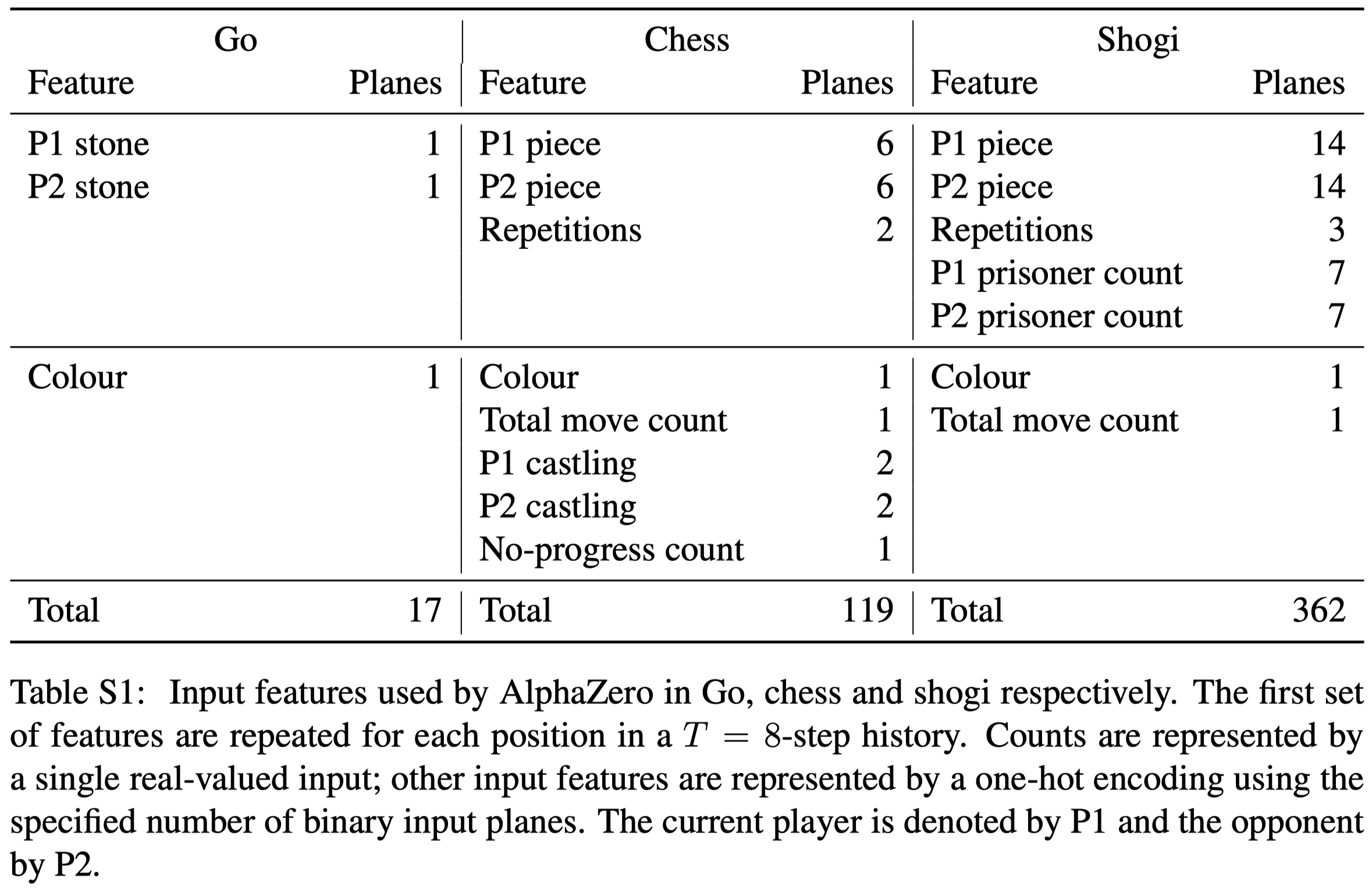
For board games, the input is an \(N\times N\times (MT+L)\) image stack that represents state using a concatenation of \(T\) sets of \(M\) planes of size \(N\times N\). Each set of planes represents the board position at a time-step \(t-T+1,\dots,t\), and is set to zero for time-steps less than \(1\). The \(M\) feature maps are composed of binary feature planes indicating the presence of the player’s pieces, with one plane for each piece type, and a second set of planes indicating the presence of the opponent’s pieces. There are additional \(L\) constant-valued planes denoting the player’s color, state of special rules, etc. The following figure summarizes input features for three board games
For Atari, the input of the representation function includes the last \(32\) RGB frames at resolution \(96\times 96\) in the range of \([0,1]\) along with the last \(32\) actions that led to each of those frames. The historical actions are encoded as an action in Atari does not necessarily have a visible effect on the observation. These actions are encoded as simple bias planes, scaled by \(a/18\), as there are \(18\) total actions in Atari.
Representation Model
For board games, the representation function uses the same architecture as AlphaZero, but with \(16\) instead of \(20\) residual blocks.
For Atari, the representation function starts with a sequence of convolutions with stride \(2\) to reduce the spatial resolution to \(6\times 6\), followed by the same ResNet as that in board games.
Dynamics Model
The input to the dynamics function is either the hidden state produced by the representation function or previous application of the dynamics function, concatenated by a representation of the action for the transition. In Atari, an action is first encoded as a one-hot vector and then tiled appropriately into \(6\times 6\times18\) planes, i.e., each feature in the one-hot vector corresponds to a plane and there are \(18\) actions in Atari games.
Interestingly, MuZero does not use as its dynamics function any memory architecture(e.g. an RNN). Instead, the dynamics function uses a ResNet similar to the representation function. I suspect this design choice mainly aims to avoid the initial state shift problem of memory architectures in off-policy training.
Actor-Critic Model
For board games, policy and value predictions use the same architecture as AlphaZero, and no reward prediction is imposed as there is no intermediate reward given.
For Atari, we represent the reward and target predictions by a categorical distribution with a discrete support set of size \(601\) with one support for every integer between \(-300\) and \(300\). The value and reward heads produce a softmax distribution over these values. During inference the value and reward predictions are computed as the expected value under their respective softmax distribution. To reduce the potential unlimited scale of the value function, the value prediction is further scaled using \(h^{-1}(x)=\text{sign}(x)\left(\left({\sqrt{1+4\epsilon(\vert x\vert +1+\epsilon)}-1\over2\epsilon}\right)^2-1\right)\) from the transformed Bellman operator, where \(\epsilon=0.001\).
Exploration
For board games, the same exploration scheme as the one described in AlphaZero is used, which adds a Dirichlet noise, at the start of each move, to the prior probabilities in the root node. For atari games, where the action space is smaller, actions are sampled from the visit count distribution parameterized using a temperature parameter \(T\):
\[\begin{align} p_a={N(a)^{1/T}\over \sum_b N(b)^{1/T}} \end{align}\]\(T\) is decayed from \(1\) for the first \(500K\) training steps to \(0.25\) at the \(1B\) steps.
Data Generation
The latest checkpoint of the network (updated every \(1000\) training steps) is used to play games with MCTS. In board games, the search is run for \(800\) simulations per move for pick an action; in Atari due to the much smaller action space \(50\) simulations per move are sufficient.
For board games, games are sent to the training job as soon as they finish. Because of much large length of Atari games, intermediate sequences are sent every \(200\) moves.
Training Process
During training, the MuZero network is unrolled for \(K=5\) hypothetical steps. Transition sequences of length \(K\) are selected by sampling a state from the replay buffer, then unrolling \(K\) steps from that state. For board games, states are sampled uniformly. In Atari, samples are drawn from a prioritized experience replay, with priority \(p_i=\vert \nu-z\vert \), where \(\nu\) is the search value and \(z\) the observed \(n\)-step return. In all experiments, we set the hyperparameters of the PER \(\alpha=\beta=1\).
Each observation \(o_t\) along the sequence also has a corresponding MCTS policy \(\pi_t\), estimated value \(\nu_t\) and environment reward \(u_t\). At each unrolled step \(k\) the network has a loss to the value, policy, reward target for that step, summed to produce the total loss for that step(see Figure S2 below). It’s interesting that MuZero does not even try to align the representations learned by the representation and the dynamics functions.
The value function is updated with the \(n\)-step bootstrapped target. For board games, we bootstrap directly to the end of the game; for Atari, we bootstrap for \(n=10\) steps into the future.
To maintain a roughly similar magnitude of gradient across different unroll steps, we scale the gradient in two separate locations:
- We scale the loss of each head by \(1\over K\) to ensure the total gradient has a similar magnitude irrespective of how many steps we unroll for.
- We also scale the gradient at the start of the dynamics function by \(1\over 2\). This ensures that the total gradient applied to the dynamics function stays constant.
To improve the learning process and bound the activations, we also scale the hidden state to the same range as the action input: \(s_{scaled}={s-\min(s)\over\max(s)-\min(s)}\). This includes both the initial state produced by the representation function and the intermediate states produced by the dynamics function, and is done channel-wise(my guess- -…)
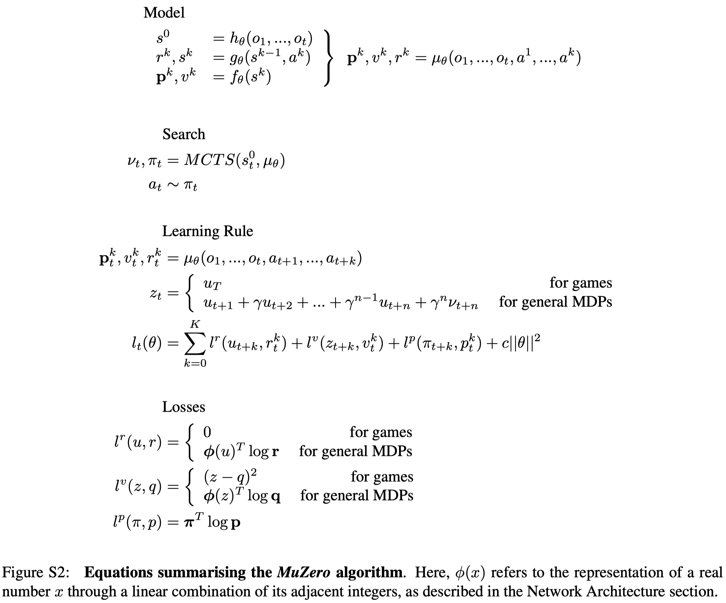
Figure S2 mathematically summarizes MuZero. Notice that
- The losses for the reward and value functions are cross entropy losses as they are represented by categorical representations.
- No off-policy correction is made. Unlike IMPALA, MuZero does not make any effort to correct the policy mismatch even though the target value is computed under a different behavior policy. I personally conjecture this is because MuZero is trained in a distributed framework with MCTS, which provides relatively high quality targets. Moreover, MuZero employs MCTS at inference, lowering the requirement of accurate prediction models
Renanalyze
To improve the sample efficiency of MuZero, the authors also introduce a variant of the algorithm, MuZero Reanalysize. MuZero Reanalyze revisits its past transitions and re-compute the policy and value target by re-executing MCTS using the latest model parameters. This provides a fresher policy and value target during training. In addition, several other hyperparameters are adjusted—primarily to increase sample reuse and avoid overfitting of the value function. Specifically, \(2.0\) samples are drawn per state, instead of \(0.1\); the value loss is weighted down to \(0.1\) compared to weights of \(1\) for policy and reward loss; and \(n\)-step return is reduced to \(n=5\) steps instead of \(n=10\) steps.
Comparison to AlphaZero
AlphaZero uses knowledge of the rules of the game in three places:
- State transitions in the search tree: During the search, the next state are produced by a perfect simulator
- Actions available at each node of the search tree: During the search, AlphaZero masks actions using the legal actions from the simulator
- Episode termination within the search tree: AlphaZero stops the search at leaf when the simulator sends the terminal value. The terminal value is backpropagated instead of the value produced by the network.
In MuZero, all of these have been replaced with the use of a single implicit model learned by a neural network:
- State transition: MuZero employs a learnable dynamics model within its search. Under this model, each node in the tree is represented by a corresponding hidden state, in which we have \(s_{k+1}=g(s_k,a_k)\).
- Actions available: MuZero only masks legal actions at the root of the search tree where the environment can be queried but does not perform any masking within the search tree. This is possible because the network rapidly learns not to predict actions that never occurred in the trajectories it is trained on.
- Terminal nodes: MuZero does not give special treatment to terminal nodes and always uses the value predicted by the network. Inside the tree, the search can proceed past a terminal node – in this case the network is expected to always predict the same value. This is achieved by treating terminal states as absorbing states during training.
In addition, Muzero is designed to operate in the general reinforcement learning setting: single-agent domains with discounted intermediate rewards of arbitrary magnitude. In contrast, AlphaZero was designed to operate in two-player games with undiscounted terminal rewards of \(\pm 1\).
Experimental Results
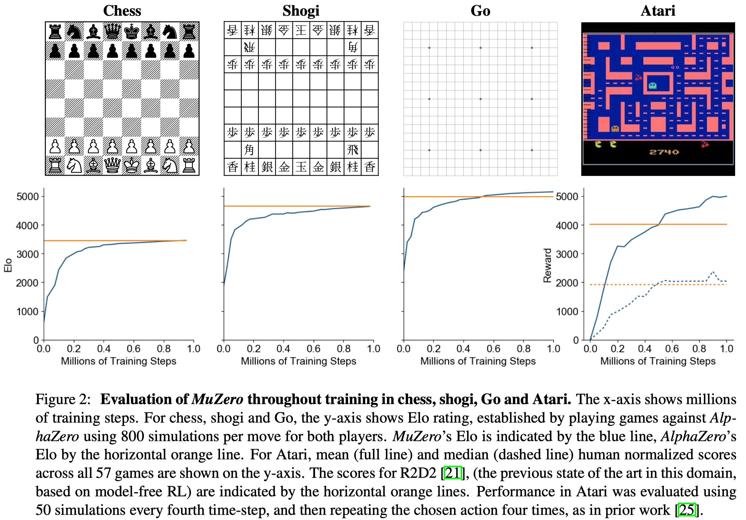
Figure 2 shows the performance throughout training in each game. MuZero slightly exceeds the performance of AlphaGo, despite using less computation per node in the search tree (\(16\) residual blocks per evaluation in MuZero compared to \(20\) blocks in AlphaGo). This suggests that MuZero may be caching its computation in the dynamics model to gain a deeper understanding of the position.
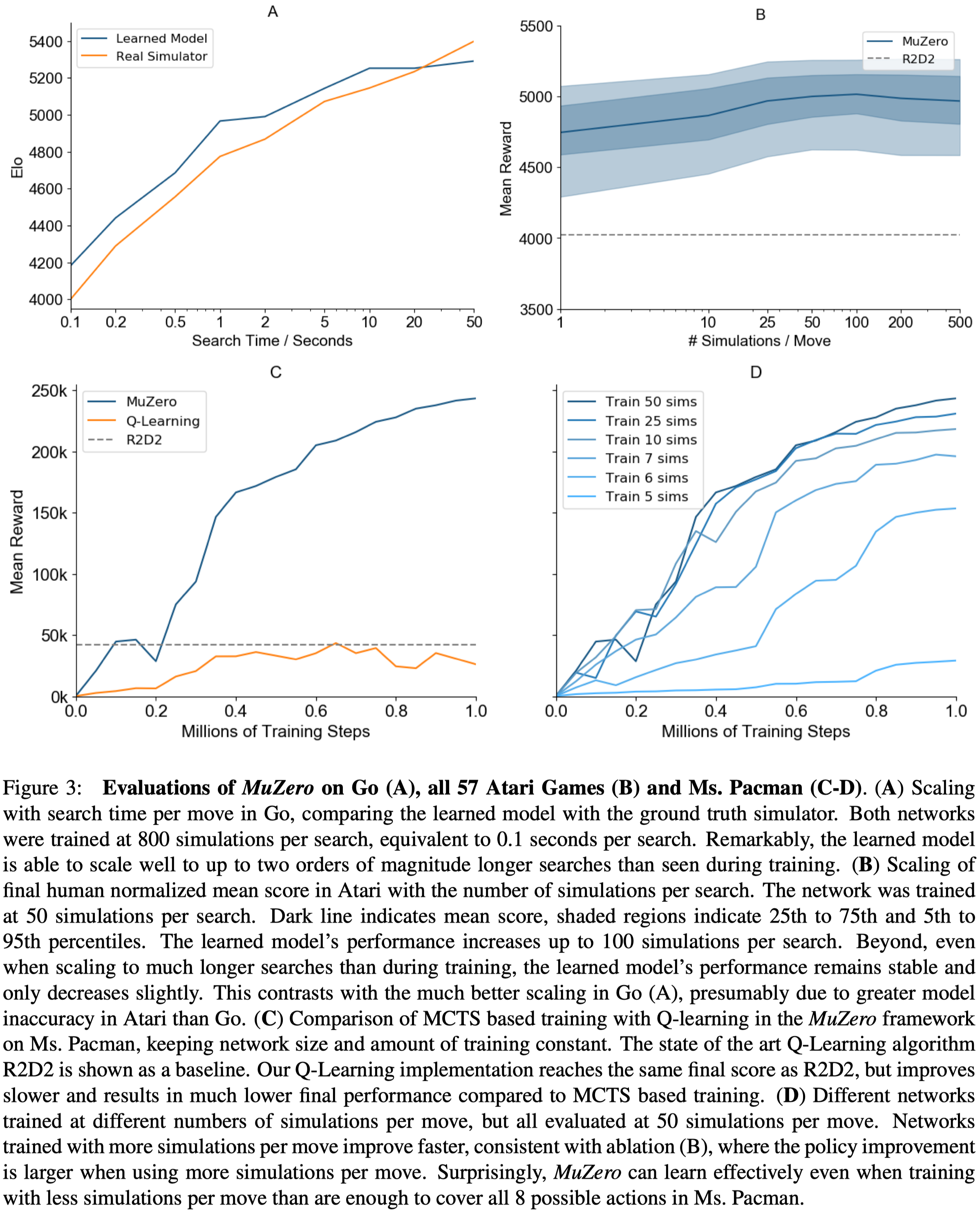
Figure 3 shows several experiments on the scalability of the planning of MuZero.
- Figure 3A shows MuZero matches the performance of a perfect model, even when doing much deeper searches (up to \(10\)s thinking time) than those from which the model was trained (around \(0.1\)s thinking time).
- Figure 3B shows that improvements in Atari due to planning are less marked than in board games, perhaps because of greater model inaccuracy; performance improves slightly with search time. On the other hand, even a single simulation—i.e. when selecting moves solely according to the learned policy—performs well, suggesting that, by the end of the training, the raw policy has learned to internalize the benefits of search.
- Figure 3C shows that even with the same network size and training steps, MuZero performs much better than Q-learning, suggesting that the search-based policy improvement step of MuZero provides a stronger learning signal than the high bias, high variance targets used by Q-learning. However, they did not analyze the effect of the categorical representation of the reward and value predictions. This may contribute to the performance of MuZero as cross-entropy loss provides a stronger learning signal than MSE.
- Figure 3D shows that the number of simulation plays an important role during training. But it’s plateaued potentially because of greater model inaccuracy as mentioned before.
References
Schrittwieser, Julian, Ioannis Antonoglou, Thomas Hubert, Karen Simonyan, Laurent Sifre, Simon Schmitt, Arthur Guez, Edward Lockhart, Demis Hassabis, Thore Graepel, Timothy Lillicrap, David Silver.” Mastering Atari, Go, Chess and Shogi by Planning with a Learned Model”