Introduction
Distributed architectures, such as Ape-X and IMPALA, have been shown to greatly boost the performance of RL algorithms in practice. Both Ape-X and IMPALA follow the design to separate the process of learning from data collection, with actors feeding experience into a buffer(or queue) and the learner receiving batches from it. In this post, we discuss a distributed method, namely Recurrent Replay Distributed DQN(R2D2) proposed by Kapturowski et al., that also follows this design pattern. This algorithm bears much resemblance to Ape-X in that it also utilizes prioritized experience replay and adopts several other improvements on DQN. The contribution of R2D2 is to incorporate recurrent architecture into Ape-X, right after the convolutional stack.
The Initial State of a Recurrent Network
To make use of a recurrent network, R2D2 stores fixed-length (\(m=120\)) sequences of \((s,a,r)\) in replay, with adjacent sequences overlapping each other by \(40\) time steps, and never crossing episode boundaries. At training time, R2D2 samples a batch of sequences and feeds them to the network. This leaves us a question, what’s an appropriate initial state for the recurrent network? Kapturowski et al. discuss four possible strategies to handle this problem:
- Trajectory replay: Replay whole episode trajectories. This avoids the problem of finding a suitable initial state but creates a number of practical, computational, and algorithmic issues due to varying and potentially environment-dependent sequence length, and higher variance of network updates because of the highly correlated nature of states in a trajectory.
- Zero state: Use a zero initial state. This basically eliminates the issues of (1), allowing independent decorrelated sampling of relatively short sequences. On the other hand, it forces the RNN to learn to recover meaningful predictions from an atypical initial state, which may limit its ability to fully rely on its recurrent state and learn to exploit long temporal correlations.
- Stored state: Store the recurrent state in the replay and use it to initialize the network at training time. This partially remedies the weakness of the zero initial state strategy, however, it may suffer from the effect of ‘representational drift’ leading to ‘recurrent state staleness’, as the stored recurrent state generated by a sufficiently old network could differ significantly from a typical state produced by a more recent version.
- Burn-in: Use a portion of the replay sequence for producing a start state, and update the network only on the remaining part of the sequence. Kapturowski et al. hypothesize that this allows the network to partially recover from a poor start state (zero, or stored but stale) and find itself in a better initial state before being required to produce accurate outputs.
Because of its weakness, trajectory replay is seldom preferable in practice. In the rest of this section, we focus on the effect of the rest three.
Effectiveness of Burn-in
The following figure demonstrates the unrolled recurrent neural network of length \(m=80\) at training time.

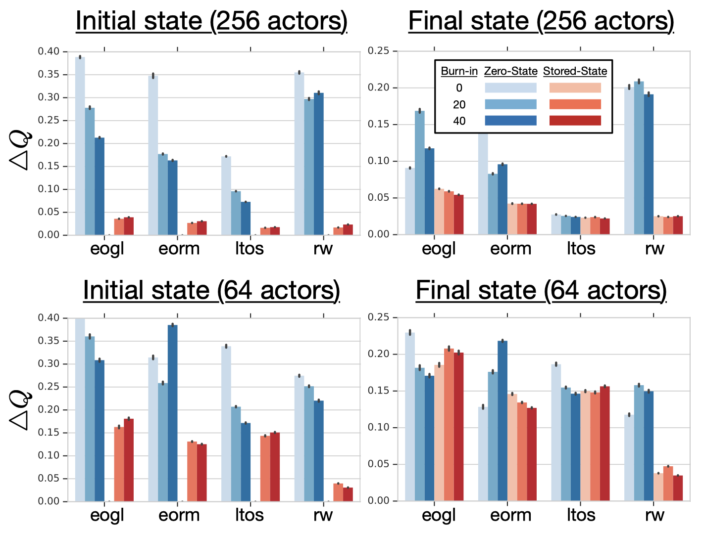
The orange part is only used to produce a start state for the blue part, and there should be no gradient back-propagated through it. The blue part is the learning part. To compensate for the missing gradient of the orange part, we overlap it with the previous sequence. The following figure demonstrates the effectiveness of burn-in, where \(\Delta Q\) is a metric defined by Kapturowski et al.—Smaller \(\Delta Q\) suggests less impact of representational shift and recurrent state staleness.

We can see that the burn-in of 20-40 steps yields better results than no burn-in. Also, notice that the representation shift is less severe in the final state than in the initial state.
Comparison between Zero State and Stored State
As for the initial state \(h_0\), the authors test both zero-state strategy and stored-state strategy, finding that the latter consistently outperforms the former. See the following figure for experimental results

Priority
Kapturowski et al. defines the priority as a mixture of max and mean absolute \(n\)-step TD-error \(\delta_i\) over the sequence: \(p=\eta\max_i\delta_i+(1-\eta)\bar\delta\), where \(\eta\), as well as priority exponent, is set to \(0.9\). This more aggressive scheme is motivated by the observation that averaging over long sequences tends to wash out large errors, thereby compressing the range of priorities and limiting the ability of prioritization to pick out useful experience.
Additional Input to RNN
The RNN in R2D2 additionally takes the previous action and reward as input.
Q-learning Loss
Another important modification to Ape-X is that R2D2 uses an invertible value function rescaling to reduce the variance of the target (refer to our post about Apex-DQfQ for more details).
\[\begin{align} h(x)&=\mathrm{sgn}(x)(\sqrt{|x|+1}-1)+\epsilon x\\\ h^{-1}(x)&=\mathrm{sgn}(x)\left(\left({\sqrt{1+4\epsilon(|x|+1+\epsilon)}-1\over 2\epsilon}\right)^2-1\right) \end{align}\]where \(\epsilon=10^{-3}\). This results in the following \(n\)-step target for the \(Q\)-value function
\[\begin{align} \hat y_t=h\left(\sum_{k=0}^{n-1}r_{t+k}\gamma^k+\gamma^nh^{-1}\Big(Q(s_{t+n},a^\*;\theta^{-})\Big)\right) \end{align}\]where \(a^*\) is the optimal action suggested by the online network, and \(\theta^-\) denotes the target network parameters which are copied from the online network parameters \(\theta\) every \(2500\) learner steps.

