NORL-HRL — Near-Optimal Representation Learning for Hierarchical Reinforcement Learning

by Sherwin Chen

10 min read May 27, 2019

Categories

• Reinforcement Learning

Tags

• Hierarchical RL
• Representation Learning

Introduction

Finally, come back to this one. Time flies :-(

This post is closely related to the previous post of HIRO. Hmm, yeah, that’s the whole introduction.

TL; DR

NORL-HRL learns a representation function $f$ and an inverse goal model $\varphi$ by maximizes the mutual information(MI) between $[s_t,\pi]$ and $s_{t+k}$,

$$\begin{align} \mathcal J(\theta, s_t,\pi)=\sum_{k=1}^c\gamma^{k-1}w_k\Big(\mathbb E_{P_\pi(s_{t+k}|s_t)}[-D(f_\theta(s_{t+k}),\varphi_\theta(s_t,\pi))]\\\ +\log\mathbb E_{\tilde s\sim\rho(s_{t+k})}\left[\exp\big(-D(f_\theta(\tilde s), \varphi_\theta(s_t,\pi))\big)\right]\Big) \end{align}$$

where $\pi$ is the lower-level policy, $D$ is a distance function(e.g., the Huber function), $f$ maps the target state $s_{t+k}$ to the goal space, $\varphi$ predicts which goal $g$ was induced by the higher-level policy such the lower-level policy $\pi$ was selected at the start state $s_t$. In practice, we replace $\pi$ with the actions taken by the lower level policy during $t$ and $t+k$, i.e., $\pi=a_{t:t+c}$. Notice that the above objective is the conditional version of MINE estimator; that’s why we said NORL-RL learns $f$ and $\varphi$ to maximize the MI between $[s_t, \pi]$ and $s_{t+k}$.

With the representation function and the inverse goal model, NORL-HRL trains the higher and lower-level policies in a similar way as HIRO except

1. The higher-level policy produces goals in the goal space, a space of lower dimension than the state space.

2. The lower-level reward function now becomes

$$\begin{align} \tilde r_k=&w_k\Big(-D(f(s_{t+k}), g)-\big(-D(f(s_{t+k}),\varphi(s_{t},\pi))-\log \mathbb E_{\tilde s\sim\rho(s_{t+k})}[\exp(-D(f_\theta(\tilde s),\varphi_\theta(s_t,\pi))]\big)\Big)\\\ where\quad w_k=&\begin{cases} 1&k<c\\\ 1-\gamma&k = c \end{cases} \end{align}$$

where $\pi=a_{t:t+c}$. Here, the first term encourages the lower-level policy to approach the goal $g$, while the second term regularizes the policy by minimizing the MI between $s_{t+k}$ and $[s_t,\pi]$.

1. NORL-HRL is more like a theoretic model for representation learning rather than an HRL algorithm. Nachum et al. only did some experiments on the representation learning part.

Framework

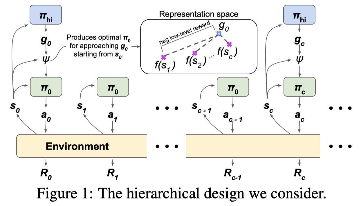
Different from HIRO, in which goals serve as a measure of dissimilarity between the current state and the desired state, goals here are used to directly produce a lower-level policy in conjunction with the current state. Formally, we use the higher-level policy to sample a goal $g_t\sim\pi^{high}(g\vert s_t)$ and translate it to a lower-level policy \(\pi^{low}t=\Psi(s_t,g_t)\), which is used to sample actions \(a{t+k}\sim\pi^{low}t(a\vert s{t+k}, k)\) for $k\in[0, c-1]$. The process is then repeated from $s_{t+c}$. (Note that the lower-level policy description in the above is a theoretical model, slightly different from the one in practice we will discuss shortly)

The mapping $\Psi$ is usually expressed as the result of an RL optimization over the policy space

$$\begin{align} \Psi(s_t,g_t)=\underset{\pi}{\arg\max}\sum_{k=1}^c\gamma^{k-1}\mathbb E_{P_\pi(s_{t+k}|s_t)}[-D(f(s_{t+k}),g_t)]\tag {1} \end{align}$$

where $P_\pi(s_{t+k}\vert s_t)$ denotes the probability of being in state $s_{t+k}$ after following lower-level policy $\pi$ for $k$ steps starting from $s_t$, $f$ denotes a representation function encoding a state to a low dimensional representation, and $D$ denotes a distance function (e.g. the Huber function), of which the negative represents the intrinsic lower-level reward. Note that $D$ here is mainly different from the one defined in HIRO in two aspects: 1) There is no $s_t$ involved since $g_t$ is no longer a measure of dissimilarity — $g_t$ now is more like the projection of $s_{t+c}$ onto the goal space. 2) The distance is now measured on the goal space (usually a lower-dimensional space) instead of the raw state space.

Good Representations Lead to Bounded Sub-Optimality

Eq.$(1)$ gives us a glimpse at what the desired lower-level policy looks like, but it does not offer any insight about how the representation learning function $f$ should be defined. Claim 4 in the paper shows that if we define $\Psi$ as a slight modification of the traditional objective given in Eq.$(1)$, then we may translate sub-optimality of $\Psi$ to a practical representation learning objective for $f$. (Do not freak out by the notations and terminologies, explanations will come shortly)

Claim 4: Let $\rho(s)$ be a prior over state space $\mathcal S$. Let $f$ and $\varphi$ be such that

$$\begin{align} \sup_{s_t,\pi}{1\over \bar w}\sum_{k=1}^c\gamma^{k-1}w_kD_{KL}(P_{\pi}(s_{t+k}|s_t)\Vert K(s_{t+k}|s_t,\pi))\le\epsilon^2/8\tag {2}\\\ where\quad K(s_{t+k}|s_t,\pi)\propto\rho(s_{t+k})\exp(-D(f(s_{t+k}),\varphi(s_t,\pi))) \end{align}$$

If the lower-level objective is defined as

$$\begin{align} \Psi(s_t,g)=\underset{\pi}{\arg\max}\sum_{k=1}^c\gamma^{k-1}w_k\mathbb E_{P_\pi(s_{t+k}|s_t)}[-D(f(s_{t+k}),g)+\log\rho(s_{t+k})-\log P_\pi(s_{t+k}|s_t)]\tag{3} \end{align}$$

then the sub-optimality of $\Psi$ is bounded by $C\epsilon$

We do not prove this claim here since the detailed proof provided by the paper is already pretty neat but still takes more than two pages. Instead, we address those notations and terminologies used above to provide some insight:

• $f$ is the representation learning function we discussed before. $\varphi$ is an auxiliary inverse goal model, which aims to predict which goal will cause $\Psi$ to yield a policy $\tilde\pi=\Psi(s,g)$ that induces subsequent distribution $P_{\tilde\pi}(s_{t+k}\vert s_t)$ similar to $P_\pi(s_{t+k}\vert s_t)$ for $k\in[1,c]$.

• We weight the KL divergence between the distributions by weights $w_k=1$ for $k<c$ and $w_k=(1-\gamma)^{-1}$ for $k=c$. We further denote $\bar w=\sum_{k=1}^c\gamma^{k-1}w_k$, which normalizes all weights so that they are summed to one.

• Nachum et al. interpret $K$ as the conditional $P(state=s’\vert repr=\varphi(s,a))$ of the joint distribution $P(state=s’)P(repr=z\vert state=s’)={1\over Z}\rho(s’)\exp(-D(f(s’),z))$ for normalization constant $Z$. In this way, we may regard $P(repr=z\vert stat=s’)$ as a Boltzmann distribution with input logits $-D(f(s’),z)$. However, although Nachum et al. claim $K$ is designed for a reason, to my best effort, I still cannot find any evidence in their proof. But as we will see later here and here, by designing $K$ in this way, we could align the representation learning to MINE and present a nice interpretation based on PGM.

• The sub-optimality of $\Psi$ measures the loss, in terms of expected value, of using policy $\Psi$ against the optimal policy. Formally, it is defined as the maximum value difference between the optimal policy $\pi^*$ and the hierarchical policy $\pi^{hier}$ learned through $\Psi$, i.e., $\mathrm{SubOpt}(\Psi)=\sup_sV^{\pi^*}(s)-V^{\pi^{hier}}(s)$.

• The lower-level objective can also be transformed into a KL

$$\Psi(s_t,\varphi(s_t,\bar\pi))=\underset{\pi}{\arg\min}\sum_{k=1}^c\gamma^{k-1}w_kD_{KL}(P_{\pi}(s_{t+k}|s_t)\Vert K(s_{t+k}|s_t,\bar\pi))\tag {4}$$

where we replace $g$ in Eq.$(3)$ with $\varphi(s_t,\bar\pi)$ and $\bar\pi$ denotes a fixed policy from which the inverse goal model produce $g$. In fact, Eq.$(4)$ is identical to the LHS of Eq.$(2)$, which brings us a nice explanation for the correlation between policy optimization and representation learning. We will come back to this in Discussion.

Put All Together

Now we develop some intuition on Claim 4. Claim 4 equally says that if we have the representation learning function $f$ and inverse goal model $\varphi$ minimizes the following loss

$$\begin{align} \underset{f,\varphi}{\arg\min}{1\over \bar w}\sum_{k=1}^c\gamma^{k-1}w_kD_{KL}(P_{\pi}(s_{t+k}|s_t)\Vert K(s_{t+k}|s_t,\pi)) \tag {2}\\\ where\quad K(s_{t+k}|s_t,\pi)\propto\rho(s_{t+k})\exp(-D(f(s_{t+k}),\varphi(s_t,\pi))) \end{align}$$

and a lower-level policy $\pi^{low}$ maximizes an RL objective with reward function defined as

$$\begin{align} \tilde r_k=&w_k\big(-D(f(s_{t+k}),g)+\log\rho(s_{t+k})-\log P_\pi(s_{t+k}|s_t)\big)\tag{3}\\\ where\quad w_k=&\begin{cases}1&if\ k\ne c\\\(1-\gamma)^{-1}&if\ k=c\end{cases} \end{align}$$

then a hierarchical policy $\pi^{hier}$ learned through $\pi^{low}$ has a bounded sub-optimality.

Now that we have grasped the overall theory, let’s dive into each part and see what they are actually doing.

Representation Learning

Let us first parameterize the representation learning function $f$ and inverse goal model $\varphi$ by $\theta$. The supremum in Eq.$(2)$ indicates that $f$ and $\varphi$ should minimize the inner part of the supremum. In practice, however, we do not have access to policy representation $\pi$. Thus, Nachum et al. propose choosing $s_t$ sampled uniformly from the replay buffer and using the subsequent $c$ actions $a_{t:t+c-1}$ as a representation of the policy. As a result, we have the representation learning objective as

$$\begin{align} \underset{\theta}{\arg\min}\ \mathcal L(\theta)&=\mathbb E_{s_t,a_{t:t+c-1}\sim\mathrm{replay}}[\mathcal L(\theta, s_t,a_{t:t+c-1})]\tag {5}\\\ where\quad \mathcal L(\theta, s_t,a_{t:t+c-1})&=\sum_{k=1}^c\gamma^{k-1}w_kD_{KL}(P_{a_{t:t+c-1}}(s_{t+k}|s_t)\Vert K(s_{t+k}|s_t,a_{t:t+c-1}))\tag {6} \end{align}$$

To simplify notation, we use $\pi=a_{t:t+c-1}$ and $E_\theta(s_{t+k},s_t,\pi)=\exp(-D(f_\theta(s_{t+k}),\varphi_\theta(s_t,\pi))$ in the following discussion. Also, recall $K_\theta(s_{t+k}\vert s_t,\pi)=\rho(s_{t+k})E_\theta(s_{t+k}, s_t, \pi)/\int \rho(s_{t+k})E_\theta(s_{t+k}, s_t, \pi)ds_{t+k}$. We now further expand Eq.$(6)$

$$\begin{align} \mathcal L(\theta, s_t,\pi)&=\sum_{k=1}^c\gamma^{k-1}w_kD_{KL}(P_{\pi}(s_{t+k}|s_t)\Vert K_\theta(s_{t+k}|s_t,\pi))\\\ &=-\sum_{k=1}^c\gamma^{k-1}w_k\mathbb E_{P_\pi(s_{t+k}|s_t)}[\log K_\theta(s_{t+k}|s_t,\pi)]\\\ &=-\sum_{k=1}^c\gamma^{k-1}w_k\Big(\mathbb E_{P_\pi(s_{t+k}|s_t)}[-D(f_\theta(s_{t+k}),\varphi_\theta(s_t,\pi))]\\\ &\qquad\qquad\qquad\qquad-\log\mathbb E_{\tilde s\sim\rho(s_{t+k})}\left[\exp\big(-D(f_\theta(\tilde s), \varphi_\theta(s_t,\pi))\big)\right]\Big)\tag {7}\\\ \end{align}$$

where we omit terms irrelevant to $\theta$ whenever possible. Note that the content in Eq.$(7)$ is similar to the objective of MINE estimator. This suggests our representation learning objective is in fact maximizing the mutual information between $[s_t,\pi]$ and $s_{t+k}$, discounting as $k$ increases. As in MINE, the gradient of the second term in brackets will introduce bias, the authors propose to replace the second term with

$$\begin{align} \mathbb E_{\tilde s\sim\rho}[E_\theta(\tilde s, s_t,\pi)]\over\mathbb E_{\tilde s\sim\mathrm{replay}}[E_\theta(\tilde s, s_t,\pi)]\tag{8} \end{align}$$

where the denominator is approximated using an additional mini-batch of states sampled from replay buffer, and there is no gradient back-propagating through it.

Since Eq.$(7)$ is essentially maximizing the mutual information between $[s_t, \pi]$ and $s_{t+k}$ for $k\in[1, c]$, other methods such as DIM may be further used to improve the performance.

lower-level Policy Learning

Eq.$(3)$ suggests optimizing a policy $\pi_{s_t,g}(a\vert s_{t+k-1},k)$ for every $s_t,g$. This is equivalent to maximizing the parameterization $\pi(a\vert s_t, g,s_{t+k},k)$. Standard RL algorithms may be employed to maximize the lower-level reward implied by

$$\begin{align} \tilde r_k=w_k\big(-D(f(s_{t+k}),g)+\log\rho(s_{t+k})-\log P_\pi(s_{t+k}|s_t)\big) \end{align}$$

where the first term in brackets is straightforward to compute but the rest terms are in general unknown. To approach this issue, we replace $P_\pi(s_{t+k}\vert s_t)$ with $K_\theta(s_{t+k}\vert s_t,\pi)$ (because of Eqs. $(5)$ and $(6)$), ending up with

$$\begin{align} \tilde r_k&=w_k\big(-D(f(s_{t+k}), g)+\log\rho(s_{t+k})-\log K_\theta(s_{t+k}|s_t,\pi)\big)\\\ &=w_k\big(-D(f(s_{t+k}), g)+D(f(s_{t+k}),\varphi(s_{t},\pi))+\log \mathbb E_{\tilde s\sim\rho(s_{t+k})}[\exp(-D(f_\theta(\tilde s),\varphi_\theta(s_t,\pi))]\big)\\\ &=w_k\Big(-D(f(s_{t+k}), g)-\big(-D(f(s_{t+k}),\varphi(s_{t},\pi))-\log \mathbb E_{\tilde s\sim\rho(s_{t+k})}[\exp(-D(f_\theta(\tilde s),\varphi_\theta(s_t,\pi))]\big)\Big)\tag {9} \end{align}$$

where $\pi$ is approximated by $a_{t:t+c-1}$ as before. Now that we have the lower-level reward computable from Eq.$(9)$, the lower-level policy can be learned as we did in HIRO using some off-policy method. (Wait, off-policy?)

Now let’s analyze our lower-level reward a bit to develop some intuition. The first term $-D(f(s_{t+k}), g)$ simply encourages the agent to reach states that is close to $g$ in the goal space; the second term $-D(f(s_{t+k}),\varphi(s_{t},\pi))-\log \mathbb E_{\tilde s\sim\rho(s_{t+k})}[\exp(-D(f_\theta(\tilde s),\varphi_\theta(s_t,\pi))]$ estimates the mutual information between $[s_t,\pi]$ and $s_{t+k}$ as we stated in the previous sub-section. By penalizing this mutual information, we are regularizing the low-policy

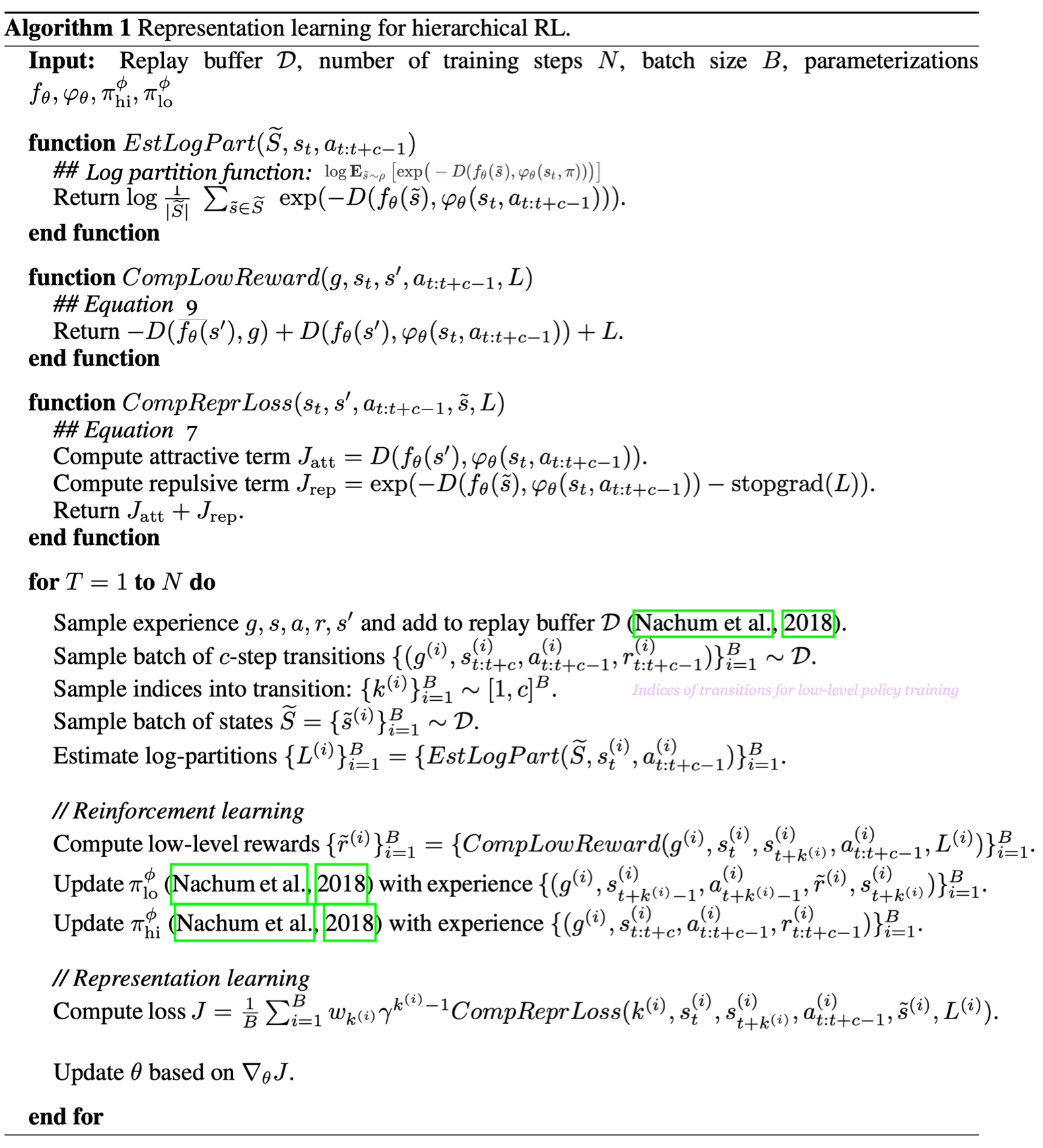
Recap and Algorithm

So far we have basically discussed everything we need to build the hierarchical algorithm. Let us do a brief review: We first compared architectures of NORL-HRL and HIRO. Then we started from claim 4, seeing how to learn good representations that lead to bounded sub-optimality and how the intrinsic reward for the lower-level policy is defined. Now it is time to present the whole algorithm

Pseudocode for NORL-HRL

Discussion

In this section, I humbly discuss some personal thinking when reading this paper.

A Different Interpretation of $K(s_{t+k}\vert s_t,\pi)\propto\rho(s_{t+k})\exp(-D(f(s_{t+k}),\varphi(s_t,\pi)))$

If we take $-D(f(s_{t+k}),\varphi(s_t,\pi))$ as reward function $r(s_t,\pi,s_{t+k})$, and relate the definition of $K$ to the probabilistic graphical model(PGM) that we’ve discussed in posts [1] [2], we may obtain the following PGM

A probabilistic graphical model for K

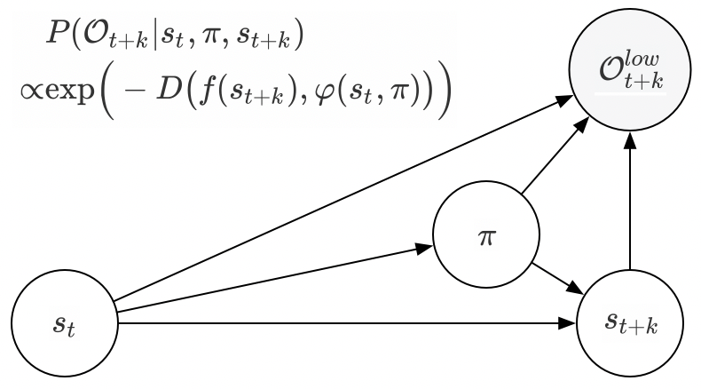
Then we have

$$\begin{align} K(s_{t+k}|s_t,\pi)=\rho(s_{t+k})P(\mathcal O_{t+k}|s_t,\pi,s_{t+k})=P(\mathcal O_{t+k},s_{t+k}|s_t,\pi) \end{align}$$

Now we may interpret $K(s_{t+k}\vert s_t,\pi)$ as the probability that state $s_{t+k}$ is optimal given the current state $s_t$ and policy $\pi$.

Correlation Between lower-level Policy Optimization and Representation Learning

As indicated by Eqs.$(4)$ and $(6)$, both lower-level policy optimization and representation learning essentially minimize the KL divergence as below if we neglect all weights and discounted factors

$$\begin{align} D_{KL}\big(P_{\pi}(s_{t+k}|s_t)\Vert K_\theta(s_{t+k}|s_t,\bar\pi)\big)\quad\forall k\in[1,c]\\\ where\quad K_\theta(s_{t+k}|s_t,\bar\pi)=\rho(s_{t+k})\exp(-D(f_\theta(s_{t+k}),\varphi_\theta(s_t,\bar\pi))) \end{align}$$

where, we take it as if $\varphi_\theta(s_t, \bar\pi)$ and $g$ are interchangeable. We can see from this KL divergence: lower-level policy optimization draws $P_{\pi}$ close to $K_\theta$, while representation learning draws $K_\theta$ close to $P_{\pi}$. Intuitively, when we optimize the lower-level policy, we want the distribution of $s_{t+k}$ under that policy to be equal to the probability of $s_{t+k}$ being optimal. On the other hand, when we do representation learning, we maximize the mutual information between $s_{t+k}$ and $[s_t,\pi]$, making the lower-level policy easier to optimize. In this regard, the representation learning plays a similar role as value function—both evaluate the current lower-level policy.

Should we relabel goals here as we do in HIRO?

This question has been haunting me for a while since it is not mentioned in the paper. So far, my personal answer is that maybe we should also do relabeling, but it is not as urgent as that is in HIRO. The same reason why HIRO requires relabeling goals still works here: as lower-level policy evolves, transition tuples collected before may no longer be valid to higher-level policy. However, this problem may, in some sense, be mitigated by the fact that we represent goals in a lower dimension.

Well, maybe the paper has mentioned that, in a very implicit way though… The experience used to train the higher-level policy includes state and lower-level action sequence, which is only useful for off-policy correction.

This question has been confirmed by Ofir Nachum: goals are indeed relabelled as in HIRO.

Is it a good idea to learn NORL-HRL in an off-policy way?

Nachum et al. propose learning NORL-HRL in an off-policy way to gain sample efficiency. However, is it really a good way to do so? Aware that we are dealing with nonstationary environments here; both higher-level and lower-level rewards are not reusable. The higher-level transitions soon becomes invalid when lower-level policy evolves, and the lower-level reward function constantly changes since it has a complex relationship with the representation learning function(through $f$), the inverse goal model(through $\varphi$), higher-level policy(through $g$), and even the lower-level policy(through $\pi$, albeit in practice, we appriximate it with actions). As a result, it may be preferable to learn these using some on-policy algorithm.

References

Mohamed Ishmael Belghazi et al. Mutual Information Neural Estimation

Ofir Nachum et al. Near-Optimal Representation Learning for Hierarchical Reinforcement Learning

Code: https://github.com/tensorflow/models/tree/master/research/efficient-hrl

Share Tweet LinkedIn Reddit